Sys.setenv(RETICULATE_PYTHON = "/home/philipp/miniconda3/envs/r-reticulate/bin/python3")
suppressPackageStartupMessages({
  library(reticulate)
  library(rtracklayer)
  library(GenomicAlignments)
  library(BRGenomics)
  library(BSgenome.Mmusculus.UCSC.mm10)
  library(tidyverse)
  library(furrr)
  library(motifmatchr)
  library(JASPAR2020)
  library(TFBSTools)
})
# Setup Multiprocessing
options(future.globals.maxSize=5000*1024^2)
future::plan(future::multisession, workers = 4)01 Prepare Input
From raw ChIP-seq data to model input.
1 Libraries
2 Configs
2.1 Output Directory
output_dir <- "/home/philipp/BPNet/input/"
if (!dir.exists(output_dir)){dir.create(output_dir)}
TFs <- c("Sox2", "Oct4", "Klf4", "Nanog")
purrr::walk(c(TFs, "patchcap", "figures"), ~ if (!dir.exists(paste0(output_dir, .x))){dir.create(paste0(output_dir, .x))})
2.2 Peak Width
As in the BPNet paper, we are using a peak width of 1000 bp, meaning we consider 500 bp up- and downstream of the ChIP-seq peaks.
peak_width <- 10002.3 Chromosome Train/Tune/Test split
all_chroms <- paste0("chr", c(1:19, "X", "Y"))

# we use the same train/tune/test split as in the BPnet paper
chrom_list <- list("tune" = c("chr2", "chr3", "chr4"), # tune set (hyperparameter tuning): chromosomes 2, 3, 4
                   "test" = c("chr1", "chr8", "chr9")) # test set (performance evaluation): chromosome 1, 8, 9
chrom_list$train <- setdiff(all_chroms, c(chrom_list$tune, chrom_list$test)) # train set: all other chromosomes
chrom_list
$tune
[1] "chr2" "chr3" "chr4"
$test
[1] "chr1" "chr8" "chr9"
$train
[1] "chr5" "chr6" "chr7" "chr10" "chr11" "chr12" "chr13" "chr14" "chr15"
[10] "chr16" "chr17" "chr18" "chr19" "chrX" "chrY" 2.4 Colors
colors = c("Klf4" = "#92C592",
           "Nanog" = "#FFE03F",
           "Oct4" = "#CD5C5C",
           "Sox2" = "#849EEB",
           "patchcap" = "#827F81")
3 Function for One-Hot Encoding
Traditionally DNA sequences are encoded using: A = [1, 0, 0, 0], C = [0, 1, 0, 0], G = [0, 0, 1, 0], T = [0, 0, 0, 1], N = [0, 0, 0, 0].
one_hot <- function(sequence) {
  len = nchar(sequence)
  mtx <- matrix(data=0, nrow=4, ncol=len)
  for (i in 1:len) {
    if (substr(sequence, i, i) == "A") mtx[1, i] = 1
    else if (substr(sequence, i, i) == "C") mtx[2, i] = 1
    else if (substr(sequence, i, i) == "G") mtx[3, i] = 1
    else if (substr(sequence, i, i) == "T") mtx[4, i] = 1
  }
  return(mtx)
}

compiler::enableJIT(0)
[1] 3one_hot_c <- compiler::cmpfun(one_hot) # compiling to bytecode not machine code like numba4 Read Stats
Look at the reading stats per TF to check how comparable the different ChIP-Nexus experiments are.
total_reads <- TFs %>%
  purrr::set_names() %>%
  purrr::map_dbl(function(tf) {
    Rsamtools::countBam(paste0("../data/chip-nexus/", tf, "/pool_filt.bam"))$records
})ggplot() +
geom_bar(aes(y=names(total_reads), x=total_reads/1e6), stat="identity", fill="blue", alpha=0.4, width=0.4) +
labs(x="N", y="TF") +
ggdark::dark_theme_linedraw()Inverted geom defaults of fill and color/colour.
To change them back, use invert_geom_defaults().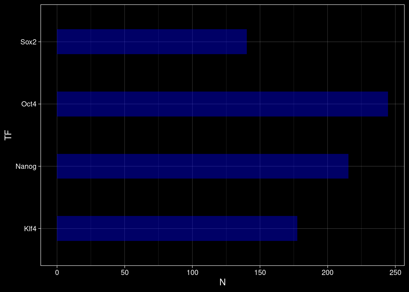
5 Load the Peak Data
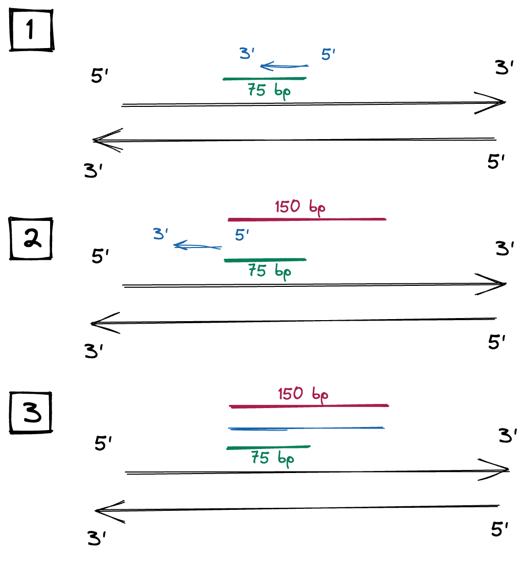
For each transcription factor (TF) we read in the peak information provided by the authors of the BPNet paper. The peaks were called using MACS2 (v.2.1.1.20160309). The following non-default settings were used: shift=-75, extsize=150, meaning the 5’ ends of each read were extended 75 bp in both directions.
In particular shift=-75 means the 5’ ends of the reads are moved -75 bp and extsize=150 means the reads are extended to a fixed length of 150 bp in 5’ -> 3’ direction.
Click to view sketch
Check the macs3 callpeak documentation here
peak_infos <- purrr::map(TFs, function(tf) {

  narrowPeaks <-
    rtracklayer::import(paste0("/home/philipp/AML_Final_Project/data/chip-nexus/", tf, "/idr-optimal-set.narrowPeak"),
                           format="narrowPeak")

  # read in the peak summits and extend symmetrically to get 1000 bp width
  summits <-
    rtracklayer::import(paste0("/home/philipp/AML_Final_Project/data/chip-nexus/", tf, "/idr-optimal-set.summit.bed"),
                           format="bed") %>%
    GenomicRanges::resize(width=peak_width, fix="center") %>%
    plyranges::mutate(TF = tf) %>%
    plyranges::mutate(set = dplyr::case_when(
                        as.character(seqnames) %in% chrom_list$tune ~ "tune",
                        as.character(seqnames) %in% chrom_list$test ~ "test",
                        as.character(seqnames) %in% chrom_list$train ~ "train"))

  GenomicRanges::elementMetadata(summits) <- cbind(
    GenomicRanges::elementMetadata(summits),
    GenomicRanges::elementMetadata(narrowPeaks)
  )

  summits

}) %>%
  do.call(what=c, args=.)

# save peak info as tsv
write_delim(data.frame(peak_infos) %>% dplyr::mutate(Region = paste0(seqnames, ":", start, "-", end)),
            file=paste0(output_dir, "region_info.tsv"), delim = "\t")

peak_infos %>% head
GRanges object with 6 ranges and 8 metadata columns:
seqnames ranges strand | TF set name
<Rle> <IRanges> <Rle> | <character> <character> <character>
[1] chrX 143482559-143483558 * | Sox2 train <NA>
[2] chrY 4149724-4150723 * | Sox2 train <NA>
[3] chr9 3001634-3002633 * | Sox2 test <NA>
[4] chr3 122145078-122146077 * | Sox2 tune <NA>
[5] chr5 28209565-28210564 * | Sox2 train <NA>
[6] chr8 86393561-86394560 * | Sox2 test <NA>
score signalValue pValue qValue peak
<numeric> <numeric> <numeric> <numeric> <integer>
[1] 1000 65.04316 37093.23 37086.70 145
[2] 1000 59.28276 2920.20 2914.44 142
[3] 1000 7.05411 2326.30 2320.59 128
[4] 1000 25.36805 1518.00 1512.39 407
[5] 1000 29.15046 1502.75 1497.15 292
[6] 1000 27.50292 1455.06 1449.46 307
-------
seqinfo: 21 sequences from an unspecified genome; no seqlengths5.1 Distribution of the MACS2 Scores
p <- peak_infos %>%
  as.data.frame() %>%
  ggplot() +
  geom_density(aes(x=log2(qValue), color=TF), alpha=0.4, fill=NA) +
  labs(x="Log2 qValue", y="Density", color="TF") +
  scale_color_manual(values=colors) +
  theme_bw()
ggsave(filename = "/home/philipp/BPNet/out/figures/macs2_scores_per_tf.pdf",
       plot = p, width = 4, height = 4)
p +
  ggdark::dark_theme_linedraw()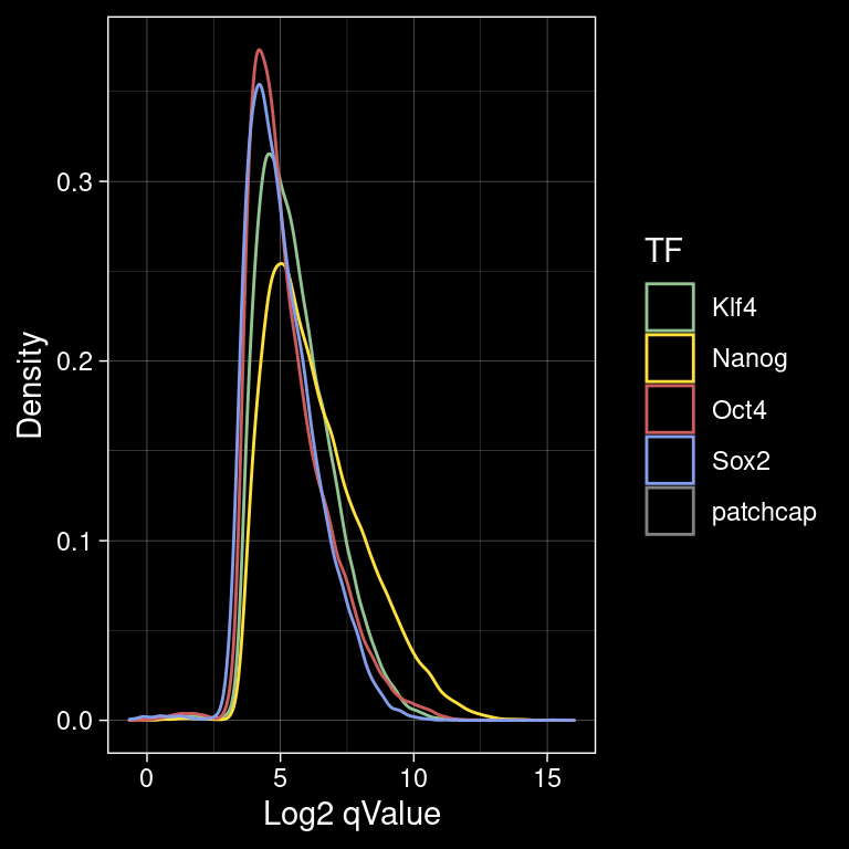
5.2 Number of Peaks per TF
p <- peak_infos %>%
  as.data.frame() %>%
  ggplot() +
  geom_bar(aes(y=TF, fill=TF), alpha=0.4, width=0.4, color="black") +
  labs(x="Number of Peaks", y="TF") +
  theme_bw() +
  scale_fill_manual(values=colors)
ggsave(filename = "/home/philipp/BPNet/out/figures/n_peaks_per_tf.pdf",
       plot = p, width = 4, height = 4)
p +
  ggdark::dark_theme_linedraw()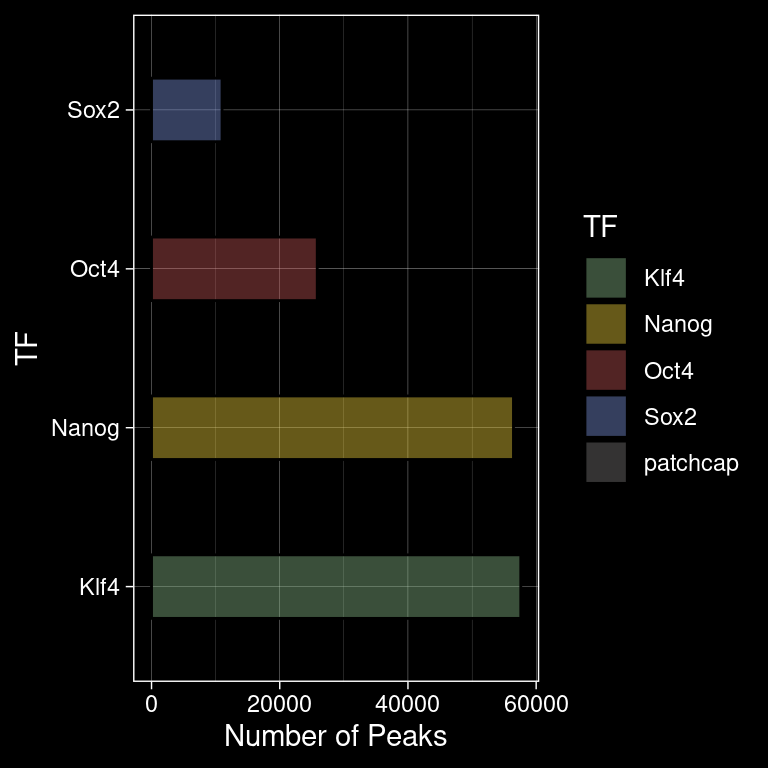
6 Translate Peak Sequences to One-Hot Encoding
seq_names <- purrr::imap(chrom_list, function(set_chroms, set_name) {

  peak_info_subset <- peak_infos[seqnames(peak_infos) %in% set_chroms]

  rnames <- paste0(as.character(peak_info_subset@seqnames), ":",
         peak_info_subset@ranges@start, "-",
         peak_info_subset@ranges@start + peak_info_subset@ranges@width - 1)

  write_lines(rnames, file = paste0(output_dir, set_name, "_seq_names.txt"))

  rnames
})str(seq_names)List of 3
$ tune : chr [1:29277] "chr3:122145078-122146077" "chr3:108433158-108434157" "chr2:52071742-52072741" "chr4:141565124-141566123" ...
$ test : chr [1:27727] "chr9:3001634-3002633" "chr8:86393561-86394560" "chr9:102205227-102206226" "chr1:134534776-134535775" ...
$ train: chr [1:93904] "chrX:143482559-143483558" "chrY:4149724-4150723" "chr5:28209565-28210564" "chr12:74803793-74804792" ...one_hot_seqs <- furrr::future_imap(chrom_list, function(set_chroms, set_name) {
peak_info_subset <- peak_infos[seqnames(peak_infos) %in% set_chroms]
peak_seqs <- BSgenome::getSeq(
BSgenome.Mmusculus.UCSC.mm10,
names=as.character(peak_info_subset@seqnames),
start=(peak_info_subset@ranges@start),
end=(peak_info_subset@ranges@start + peak_width - 1),
strand="+"
)
peak_seqs@ranges@NAMES <- seq_names[[set_name]]
# check for correctness here: https://genome.ucsc.edu/cgi-bin/hgTracks?db=mm10
Biostrings::writeXStringSet(x=peak_seqs,
filepath = paste0(output_dir, set_name, "_seqs.fa"))
# one hot encode the sequence
one_hot_mtx <- matrix(data=0, nrow=length(peak_seqs)*4, ncol=peak_width)
for (peak_index in 1:length(peak_seqs)) {
one_hot_mtx[(((peak_index-1)*4)+1):((peak_index)*4), ] <-
one_hot_c(as.character(peak_seqs[[peak_index]]))
}
one_hot_mtx
})Check the output:
str(one_hot_seqs)List of 3
$ tune : num [1:117108, 1:1000] 1 0 0 0 0 1 0 0 0 0 ...
$ test : num [1:110908, 1:1000] 0 0 0 1 0 1 0 0 0 0 ...
$ train: num [1:375616, 1:1000] 0 0 0 1 1 0 0 0 0 1 ...Write the matrices in binary format to disk using reticulate.
import numpy as np

for key, val in r.one_hot_seqs.items():
  old_shape = val.shape
  val = val.reshape(int(val.shape[0]/4), 4, 1000).astype(np.float32)
  print(f"{key}: {old_shape} -> {val.shape}")
  save_path = f"{r.output_dir}{key}_one_hot_seqs.npy"
  print(f"-> {save_path}")
  np.save(file=save_path, arr=val)
tune: (117108, 1000) -> (29277, 4, 1000)
-> /home/philipp/BPNet/input/tune_one_hot_seqs.npy
test: (110908, 1000) -> (27727, 4, 1000)
-> /home/philipp/BPNet/input/test_one_hot_seqs.npy
train: (375616, 1000) -> (93904, 4, 1000)
-> /home/philipp/BPNet/input/train_one_hot_seqs.npy7 Extract the TF Counts
First we have to merge overlapping peaks from the peak info file. Otherwise we read reads aligning to these overlapping peaks several times.
peak_infos_reduced <- GenomicRanges::reduce(resize(peak_infos, GenomicRanges::width(peak_infos + 1), "start"))
peak_infos_reduced
GRanges object with 85250 ranges and 0 metadata columns:
seqnames ranges strand
<Rle> <IRanges> <Rle>
[1] chrX 5704156-5705557 *
[2] chrX 6278899-6280002 *
[3] chrX 6411759-6412760 *
[4] chrX 6415698-6416699 *
[5] chrX 6445022-6446023 *
... ... ... ...
[85246] chr10 130523572-130524574 *
[85247] chr10 130527565-130528566 *
[85248] chr10 130535527-130536528 *
[85249] chr10 130541495-130543475 *
[85250] chr10 130594405-130595406 *
-------
seqinfo: 21 sequences from an unspecified genome; no seqlengths### Parallel loop over all tfs
tf_counts <- TFs %>%
purrr::set_names() %>%
furrr::future_map(function(tf) {
# read only from the alignment file in the given peak regions
# note: make sure that the BAM file is sorted (check for presence of ".bam.bai")
alignments <- readGAlignments(paste0("../data/chip-nexus/", tf, "/pool_filt.bam"),
param = ScanBamParam(which=peak_infos_reduced))
# split the alignment into pos and neg strand
align_pos <- alignments[GenomicRanges::strand(alignments)=="+"]
align_neg <- alignments[GenomicRanges::strand(alignments)=="-"]
# only retain first base pair of each read
align_pos@cigar <- rep("1M", length(align_pos))
align_neg@start <- GenomicAlignments::end(align_neg)
align_neg@cigar <- rep("1M", length(align_neg))
# compute the coverage per base pair
cov_list = list("pos" = GenomicAlignments::coverage(align_pos, weight = 1L),
"neg" = GenomicAlignments::coverage(align_neg, weight = 1L))
chrom_list %>%
purrr::imap(function(set_chroms, set_name) {
peak_info_subset <- peak_infos[seqnames(peak_infos) %in% set_chroms]
c("pos", "neg") %>%
purrr::set_names() %>%
purrr::map(function(strand) {
mtx <- matrix(data=0, ncol=peak_width, nrow=length(peak_info_subset))
for (i in 1:length(peak_info_subset)) {
chr <- as.character(peak_info_subset[i]@seqnames)
position_index <- peak_info_subset[i]@ranges@start:(peak_info_subset[i]@ranges@start + peak_width - 1)
mtx[i, ] = as.numeric(cov_list[[strand]][[chr]][position_index])
}
mtx
})
})
})str(tf_counts)List of 4
$ Sox2 :List of 3
..$ tune :List of 2
.. ..$ pos: num [1:29277, 1:1000] 0 0 0 0 0 0 0 0 1 0 ...
.. ..$ neg: num [1:29277, 1:1000] 0 0 1 0 0 0 0 0 1 0 ...
..$ test :List of 2
.. ..$ pos: num [1:27727, 1:1000] 0 0 0 0 0 0 0 0 0 0 ...
.. ..$ neg: num [1:27727, 1:1000] 0 0 0 0 0 0 0 1 0 0 ...
..$ train:List of 2
.. ..$ pos: num [1:93904, 1:1000] 0 0 0 0 0 0 0 0 0 0 ...
.. ..$ neg: num [1:93904, 1:1000] 0 0 0 0 0 0 0 0 0 0 ...
$ Oct4 :List of 3
..$ tune :List of 2
.. ..$ pos: num [1:29277, 1:1000] 1 1 1 0 0 0 0 0 0 0 ...
.. ..$ neg: num [1:29277, 1:1000] 1 0 1 0 0 0 0 0 0 0 ...
..$ test :List of 2
.. ..$ pos: num [1:27727, 1:1000] 0 0 0 0 0 0 0 0 0 0 ...
.. ..$ neg: num [1:27727, 1:1000] 0 0 0 0 0 2 0 0 0 0 ...
..$ train:List of 2
.. ..$ pos: num [1:93904, 1:1000] 0 0 0 0 0 0 0 0 2 0 ...
.. ..$ neg: num [1:93904, 1:1000] 0 0 1 0 0 0 0 0 0 0 ...
$ Klf4 :List of 3
..$ tune :List of 2
.. ..$ pos: num [1:29277, 1:1000] 0 0 1 0 0 0 0 0 0 0 ...
.. ..$ neg: num [1:29277, 1:1000] 0 0 0 0 0 0 0 0 0 0 ...
..$ test :List of 2
.. ..$ pos: num [1:27727, 1:1000] 0 1 0 0 0 0 0 0 0 0 ...
.. ..$ neg: num [1:27727, 1:1000] 0 0 0 0 0 3 0 0 0 0 ...
..$ train:List of 2
.. ..$ pos: num [1:93904, 1:1000] 0 0 0 0 0 1 0 0 2 0 ...
.. ..$ neg: num [1:93904, 1:1000] 0 0 0 0 0 0 0 0 0 0 ...
$ Nanog:List of 3
..$ tune :List of 2
.. ..$ pos: num [1:29277, 1:1000] 1 0 1 0 0 0 0 0 0 0 ...
.. ..$ neg: num [1:29277, 1:1000] 0 0 0 0 0 0 0 0 0 0 ...
..$ test :List of 2
.. ..$ pos: num [1:27727, 1:1000] 0 1 0 1 0 0 0 0 0 0 ...
.. ..$ neg: num [1:27727, 1:1000] 0 1 0 0 0 1 0 1 0 0 ...
..$ train:List of 2
.. ..$ pos: num [1:93904, 1:1000] 0 0 0 0 0 0 0 0 0 0 ...
.. ..$ neg: num [1:93904, 1:1000] 0 0 0 0 0 0 0 0 0 0 ...Write the matrices in binary format to disk using reticulate.
import numpy as np

for tf_name, tf_entry in r.tf_counts.items():
  print(tf_name)
  for set_name, set_entry in tf_entry.items():
    mtx = np.stack([set_entry["pos"], set_entry["neg"]], axis=1).astype(np.float32)
    print(f"\t{set_name} shape: {mtx.shape}")
    save_path = f"{r.output_dir}{tf_name}/{set_name}_counts.npy"
    print(f"\t-> {save_path}")
    np.save(file=save_path, arr=mtx)
Sox2
tune shape: (29277, 2, 1000)
-> /home/philipp/BPNet/input/Sox2/tune_counts.npy
test shape: (27727, 2, 1000)
-> /home/philipp/BPNet/input/Sox2/test_counts.npy
train shape: (93904, 2, 1000)
-> /home/philipp/BPNet/input/Sox2/train_counts.npy
Oct4
tune shape: (29277, 2, 1000)
-> /home/philipp/BPNet/input/Oct4/tune_counts.npy
test shape: (27727, 2, 1000)
-> /home/philipp/BPNet/input/Oct4/test_counts.npy
train shape: (93904, 2, 1000)
-> /home/philipp/BPNet/input/Oct4/train_counts.npy
Klf4
tune shape: (29277, 2, 1000)
-> /home/philipp/BPNet/input/Klf4/tune_counts.npy
test shape: (27727, 2, 1000)
-> /home/philipp/BPNet/input/Klf4/test_counts.npy
train shape: (93904, 2, 1000)
-> /home/philipp/BPNet/input/Klf4/train_counts.npy
Nanog
tune shape: (29277, 2, 1000)
-> /home/philipp/BPNet/input/Nanog/tune_counts.npy
test shape: (27727, 2, 1000)
-> /home/philipp/BPNet/input/Nanog/test_counts.npy
train shape: (93904, 2, 1000)
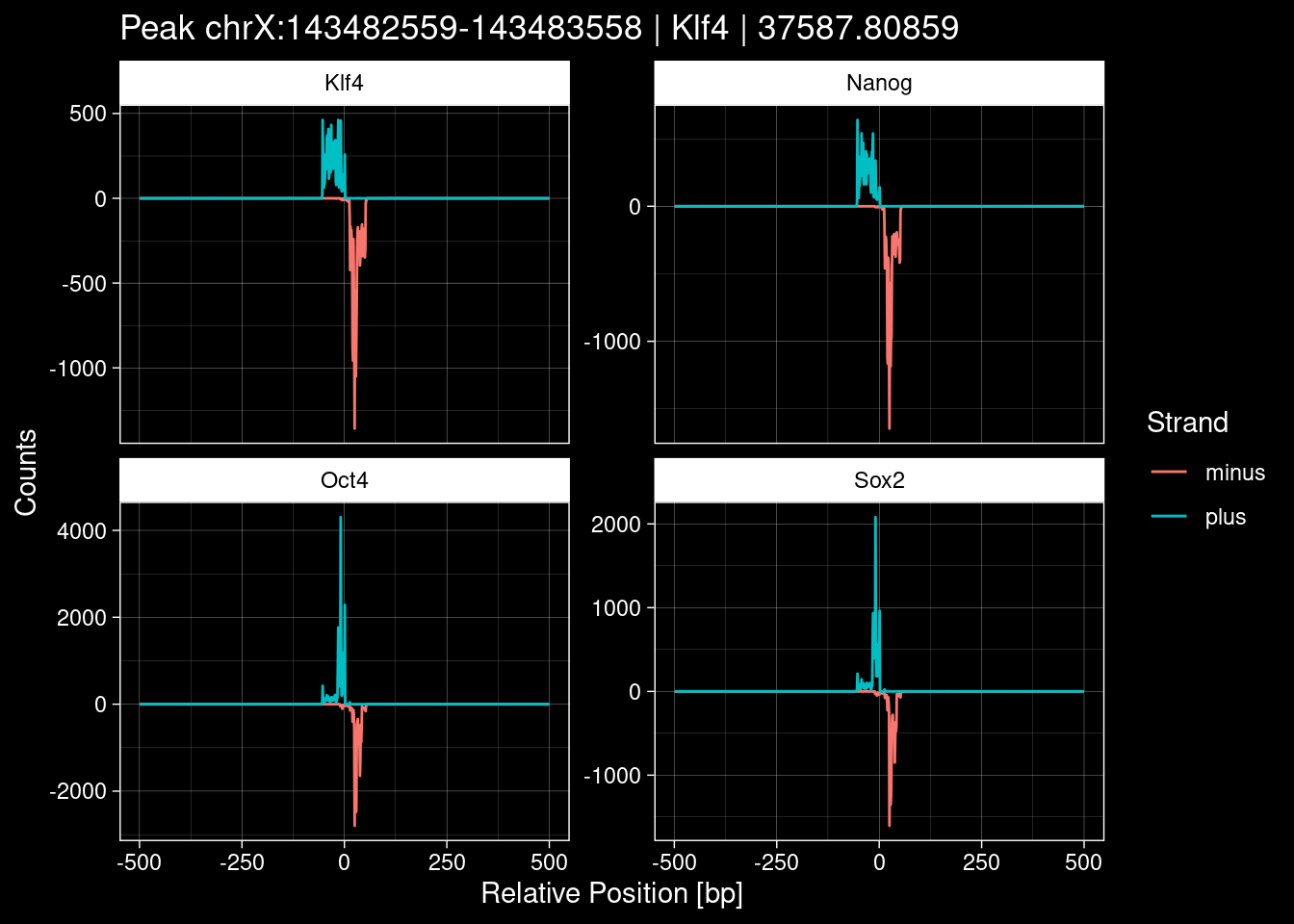
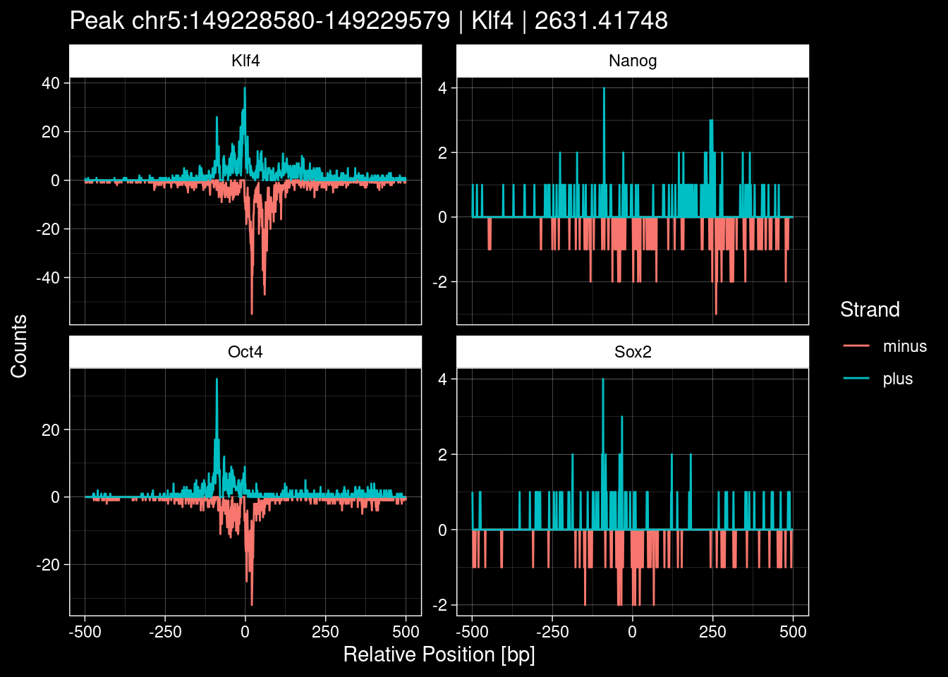
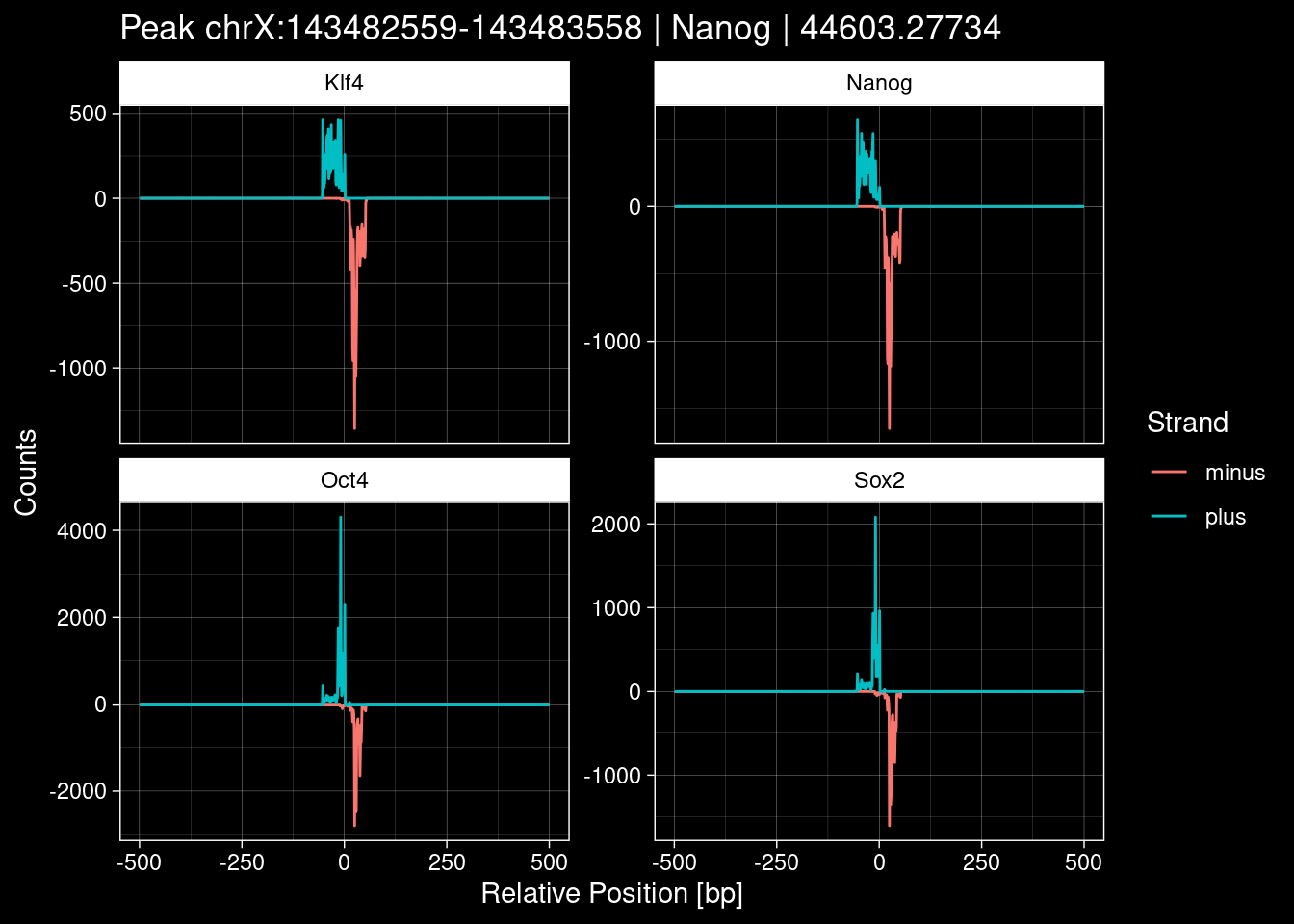
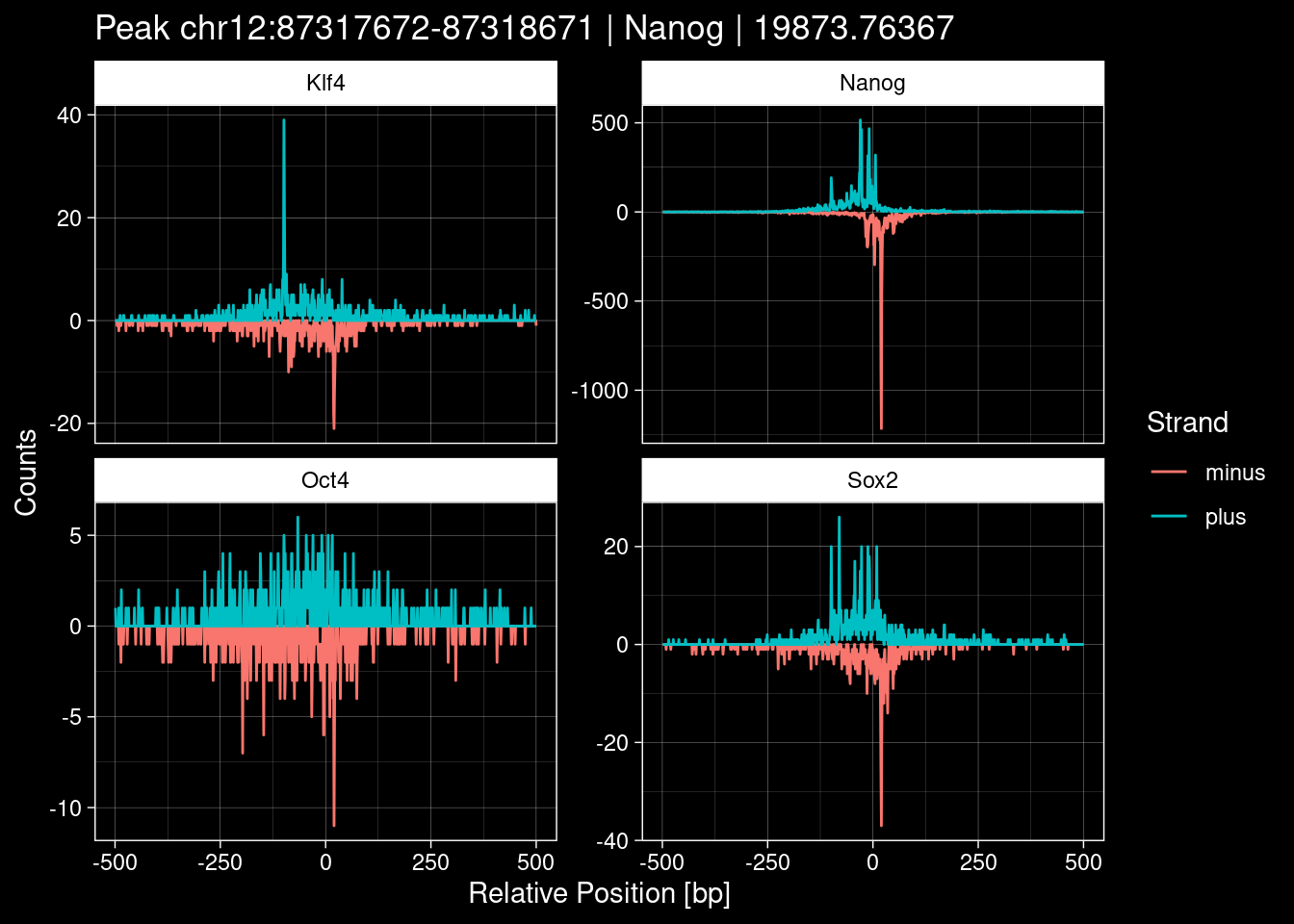
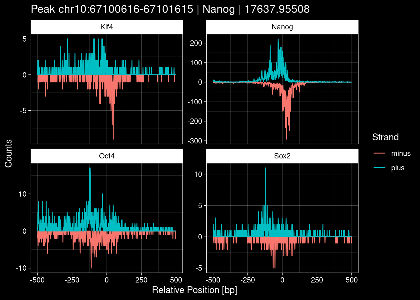
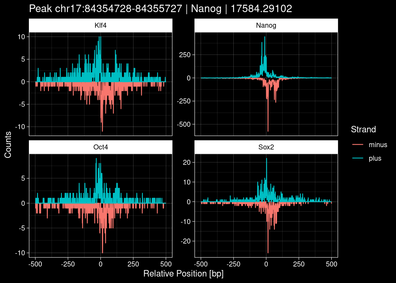
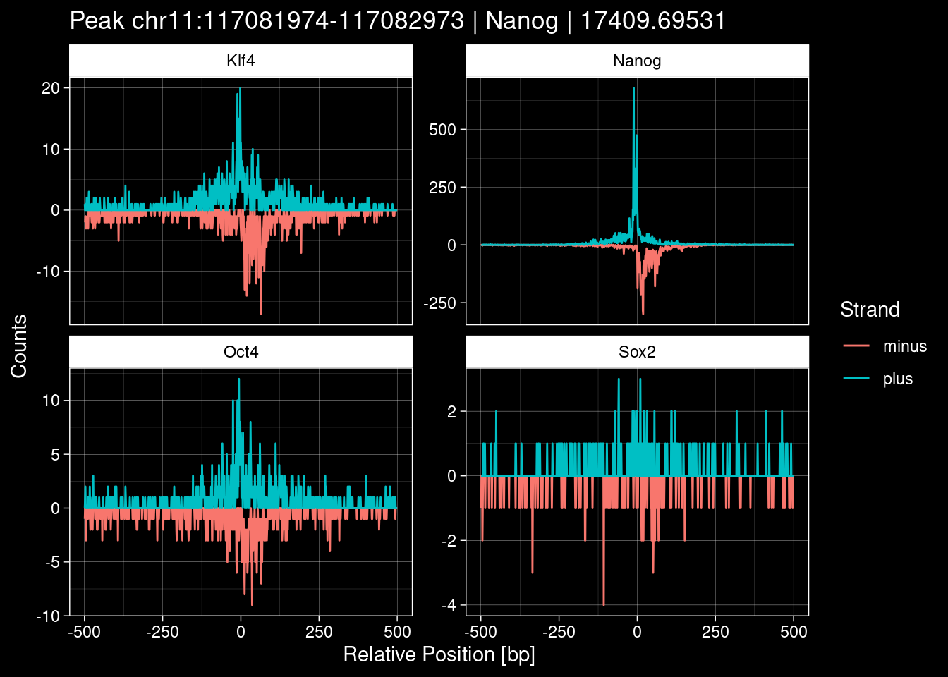
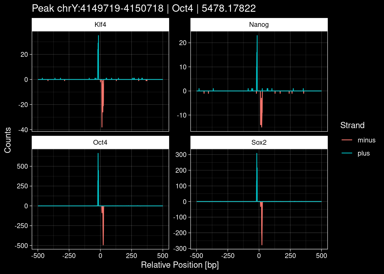
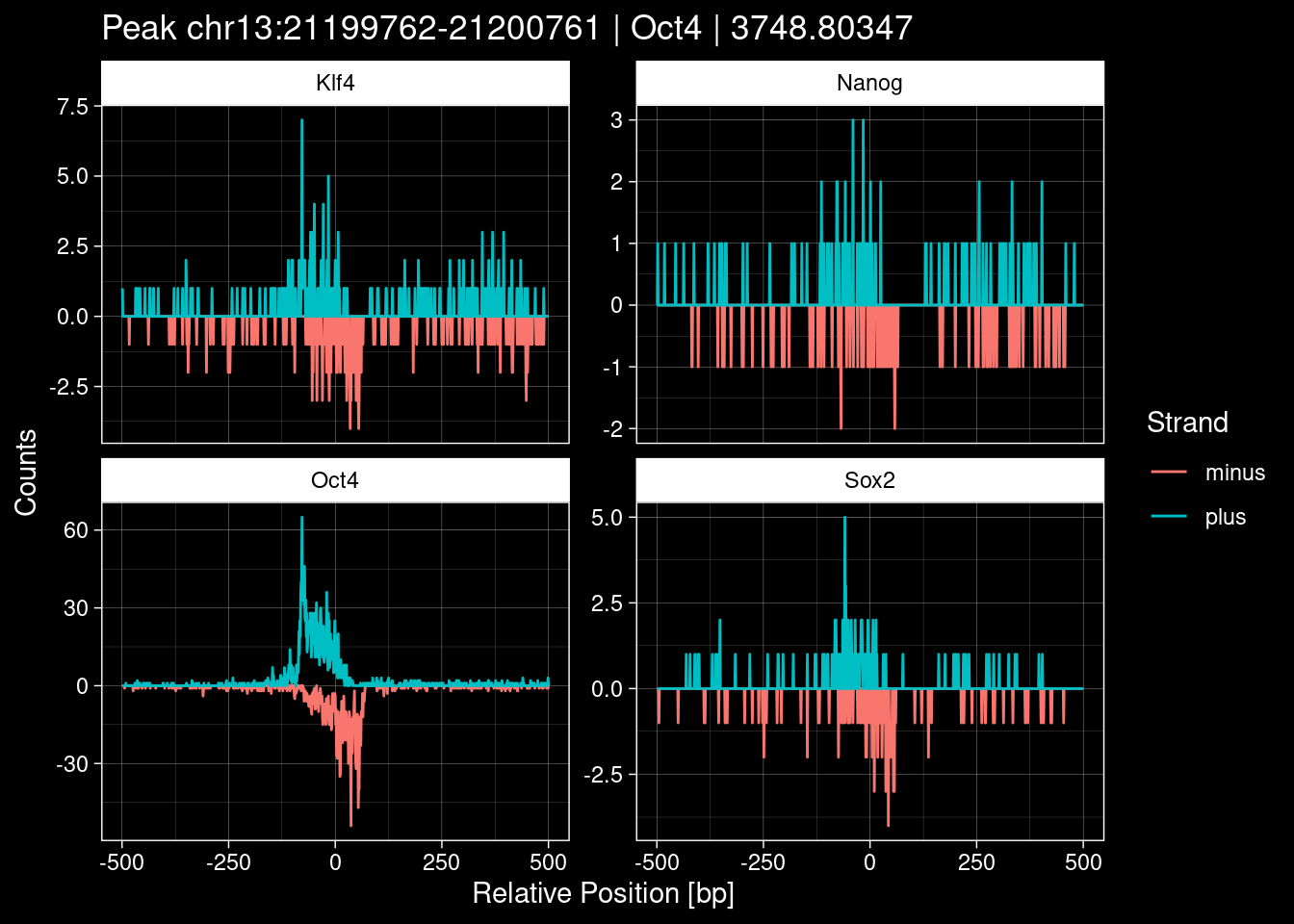
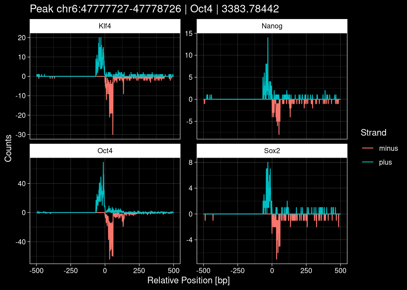
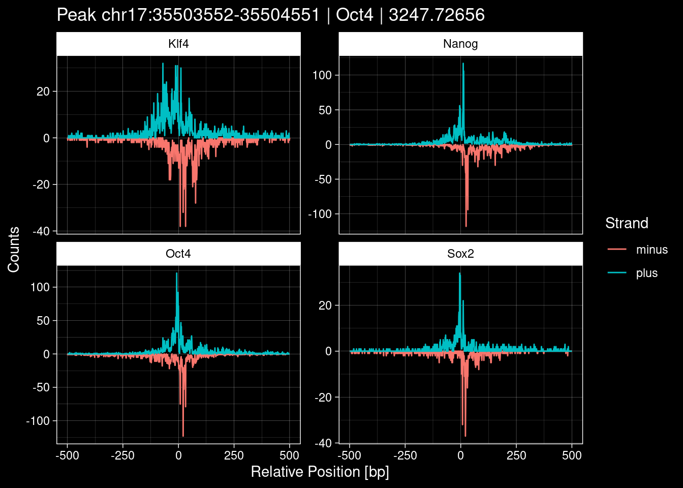
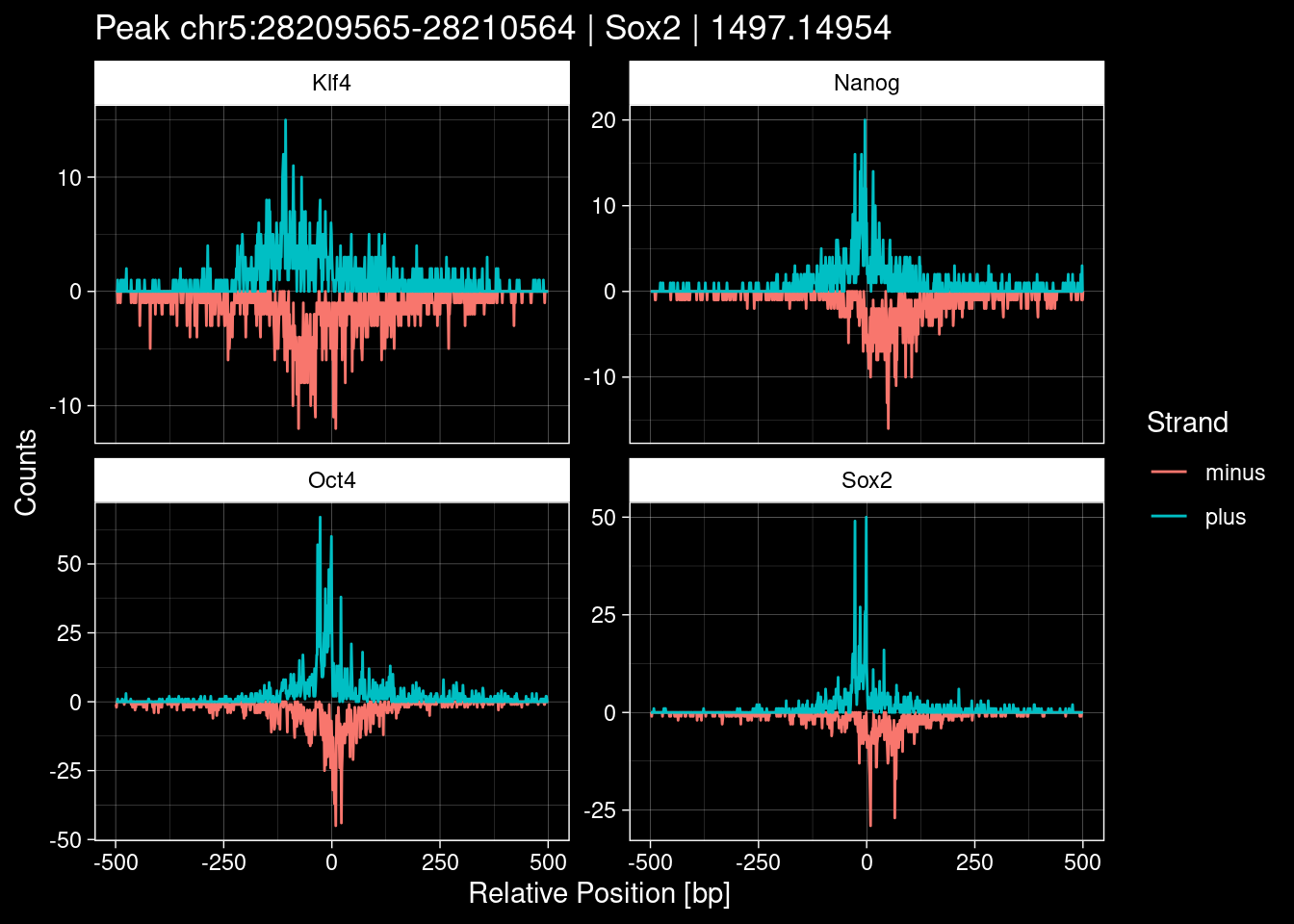
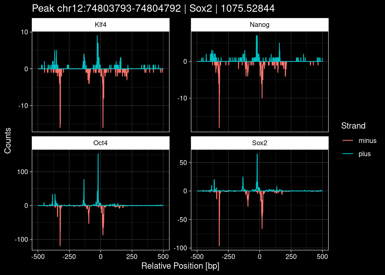
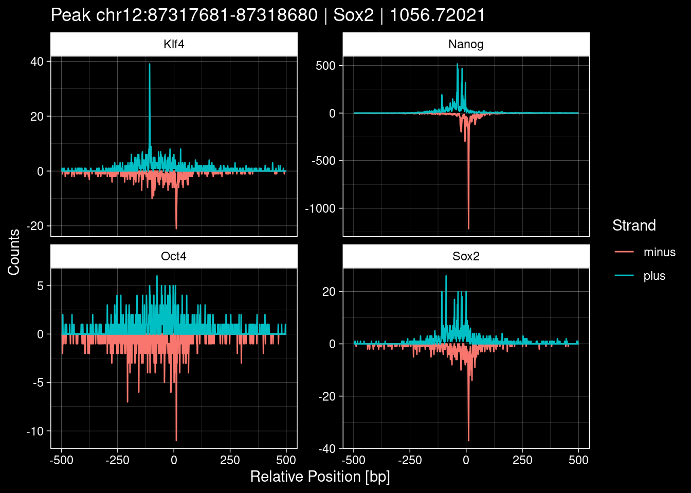
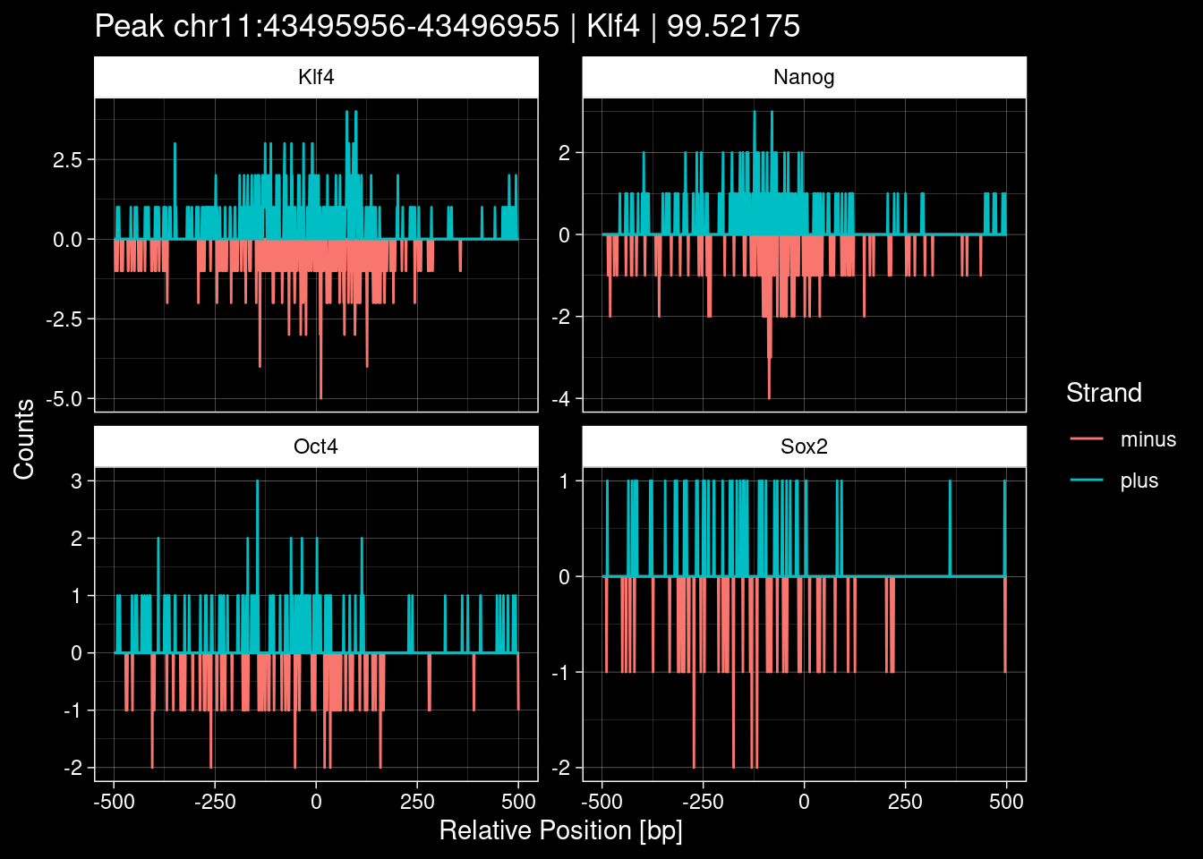
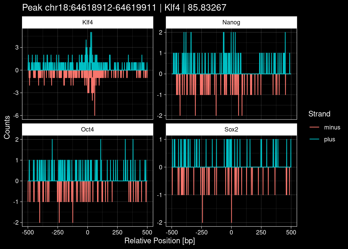
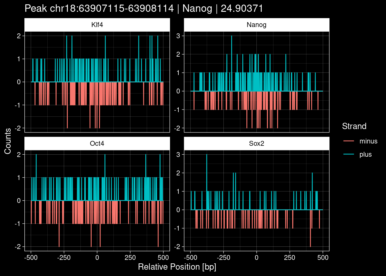
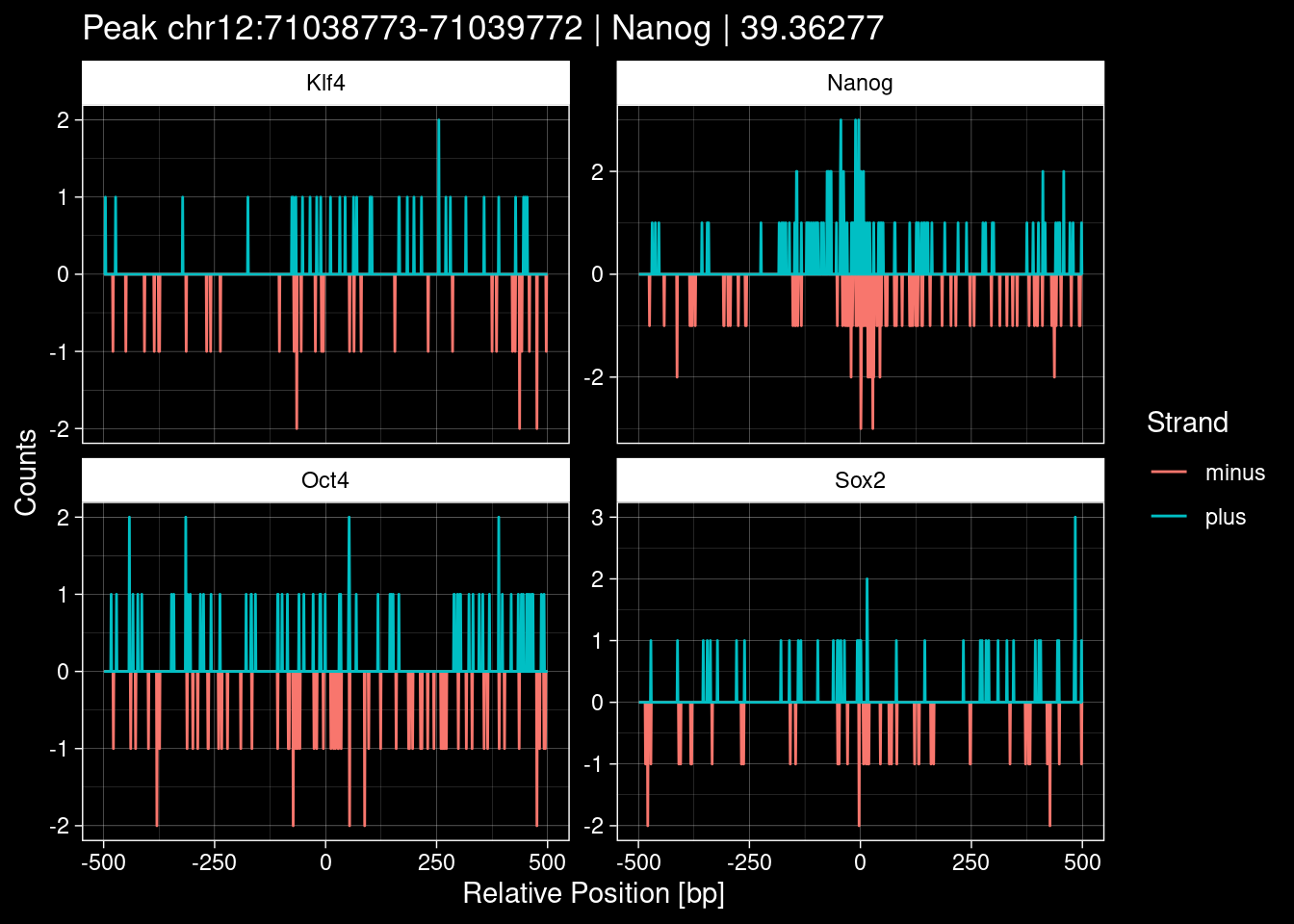
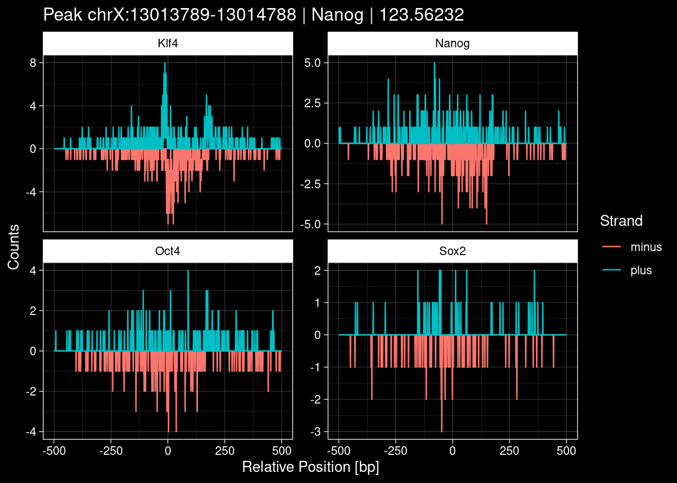
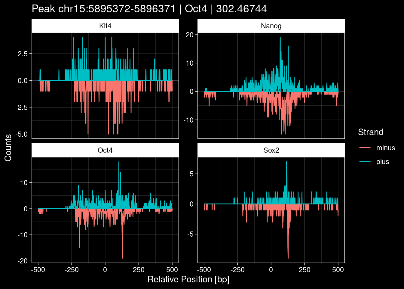
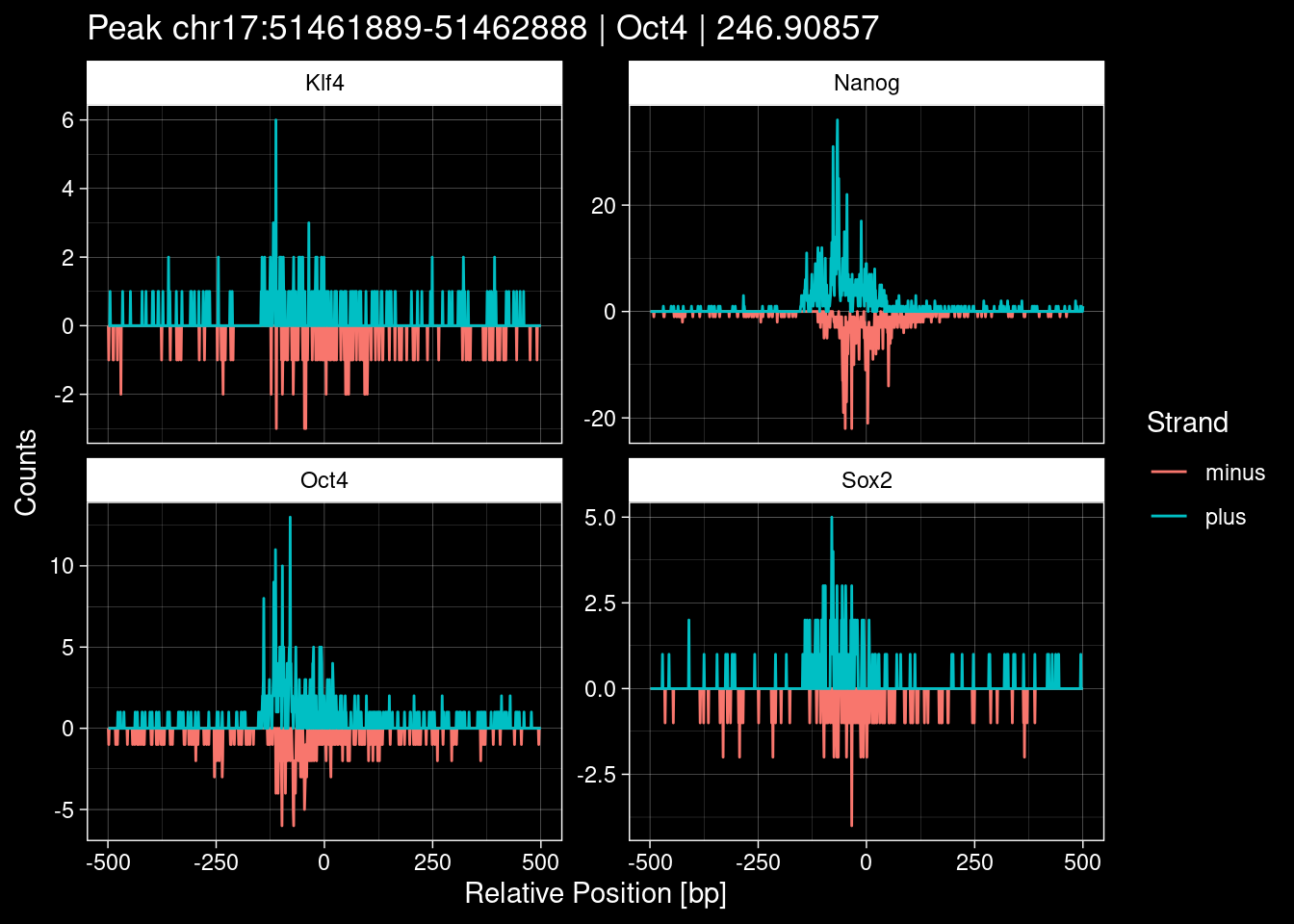
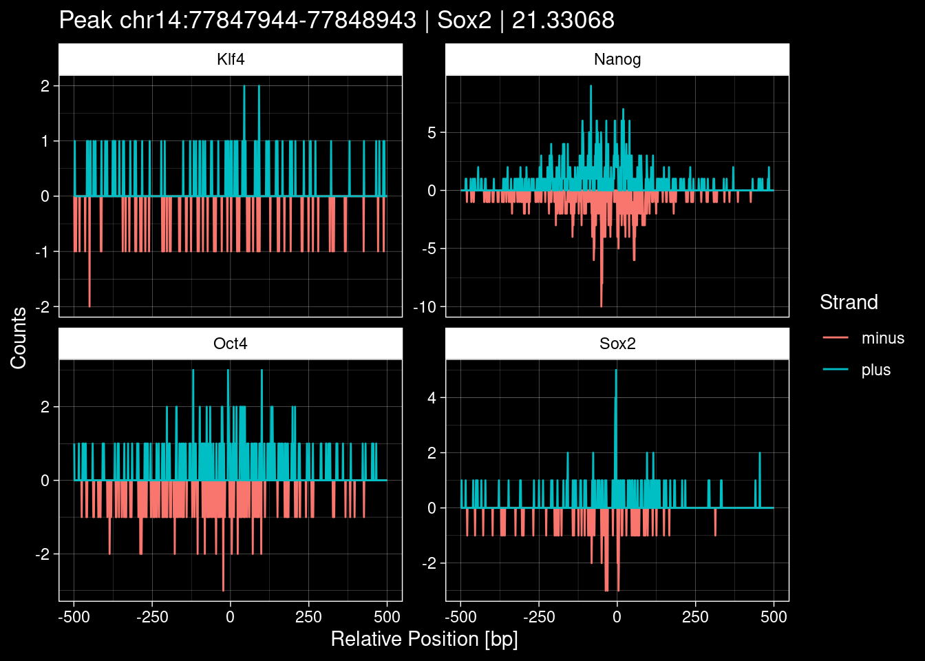
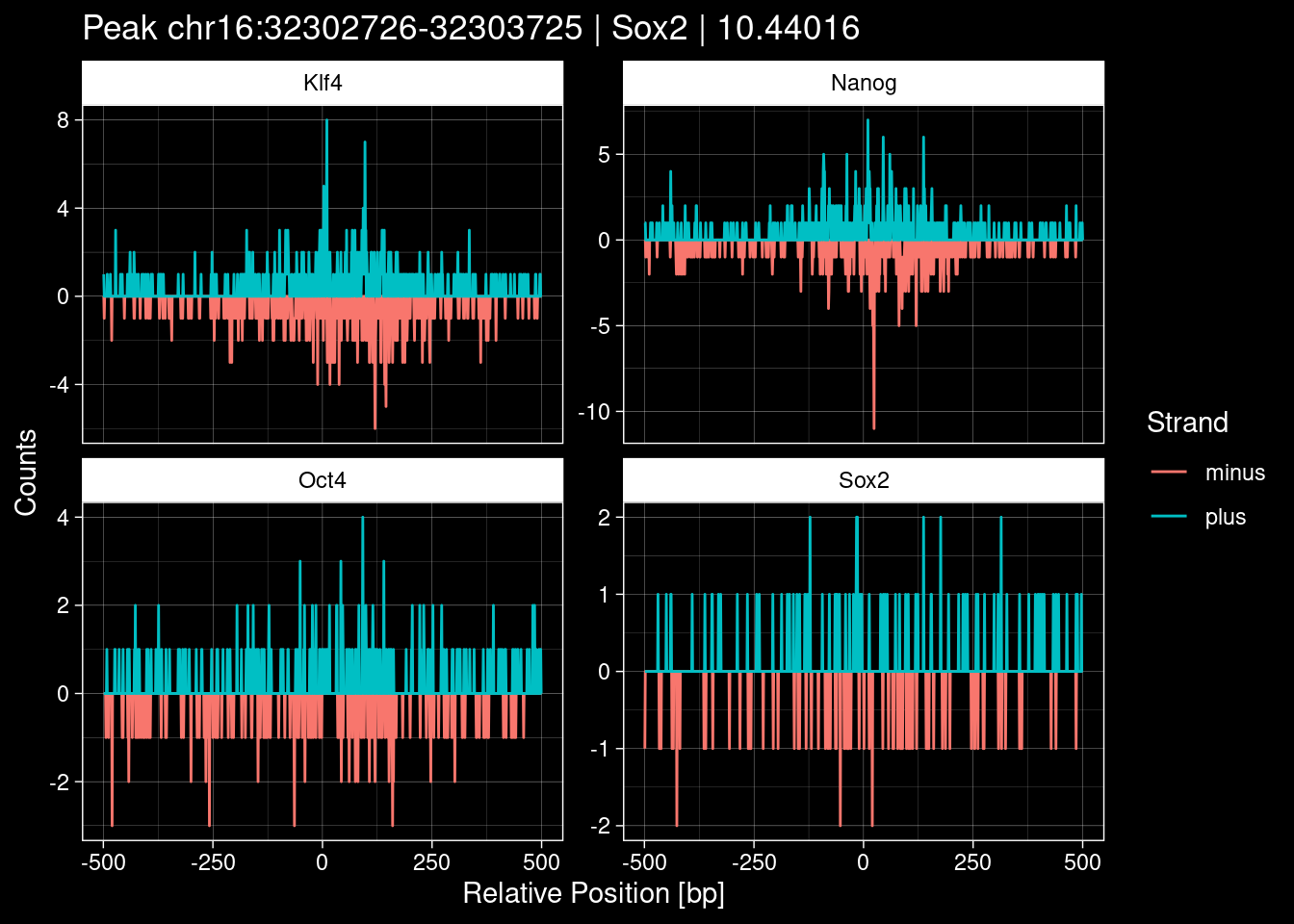
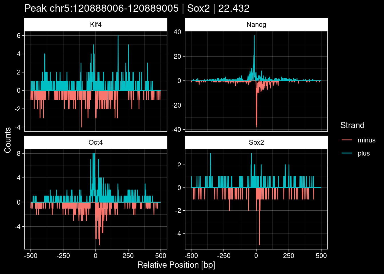
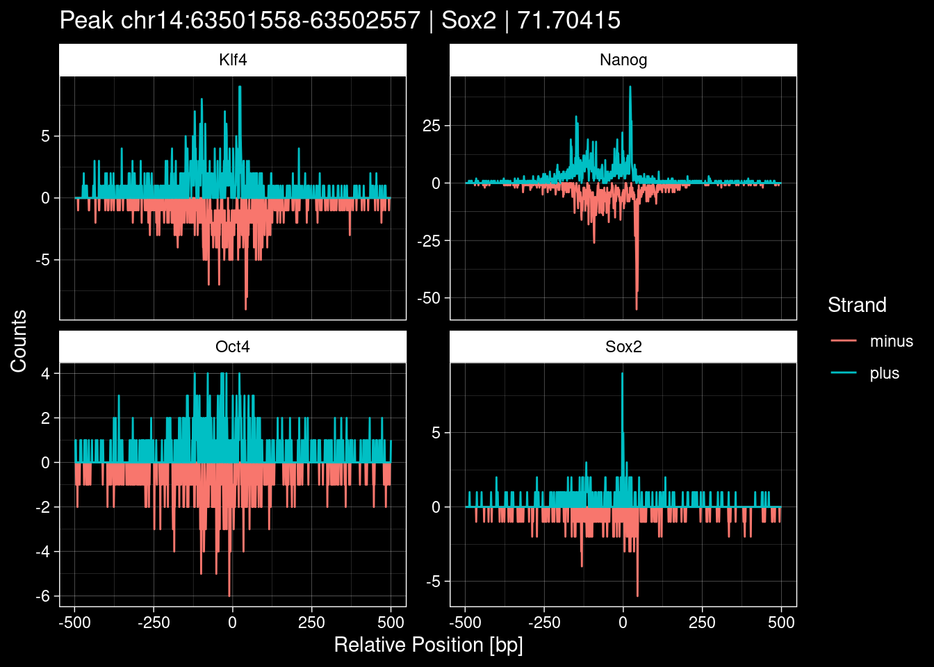
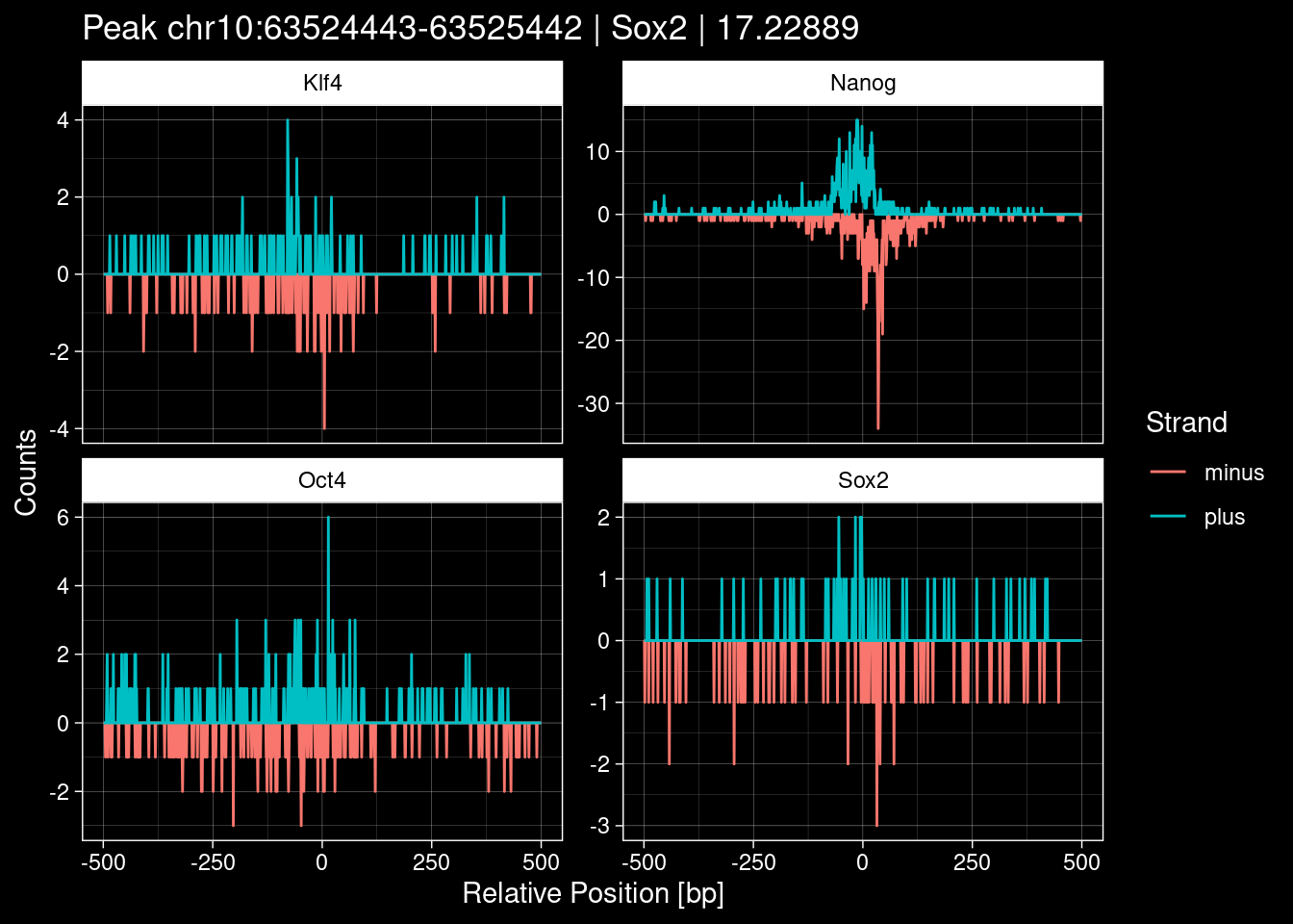
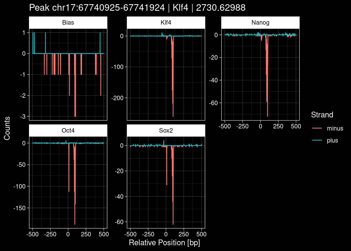
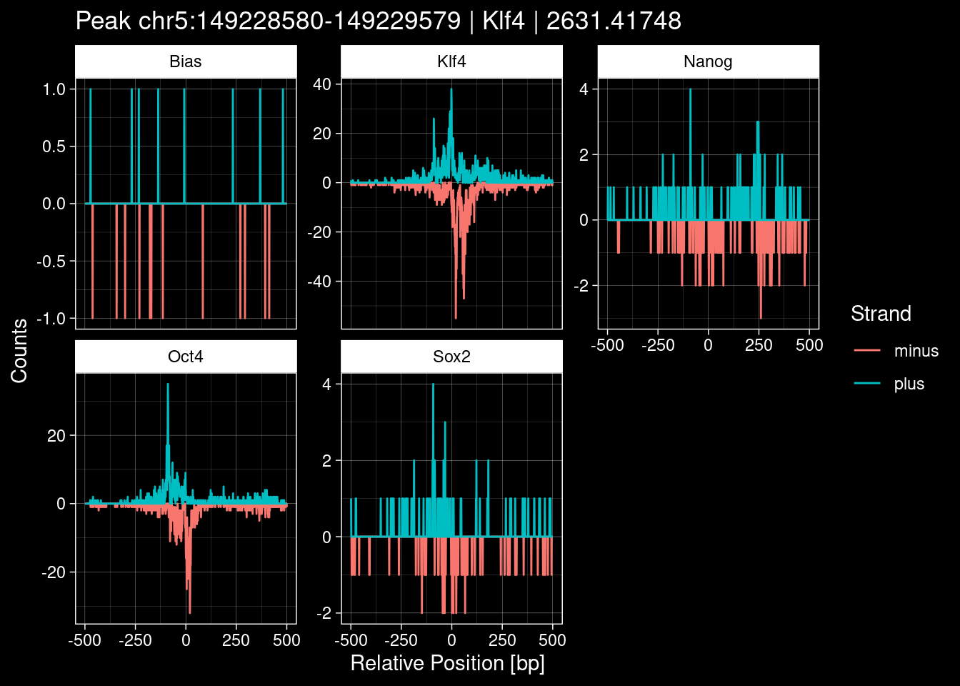
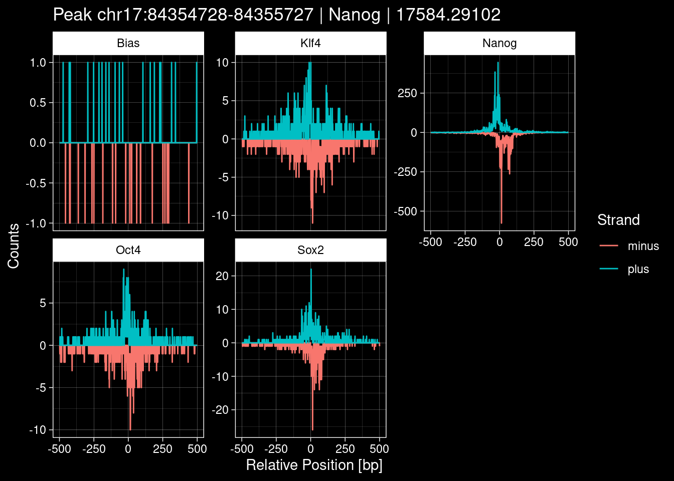
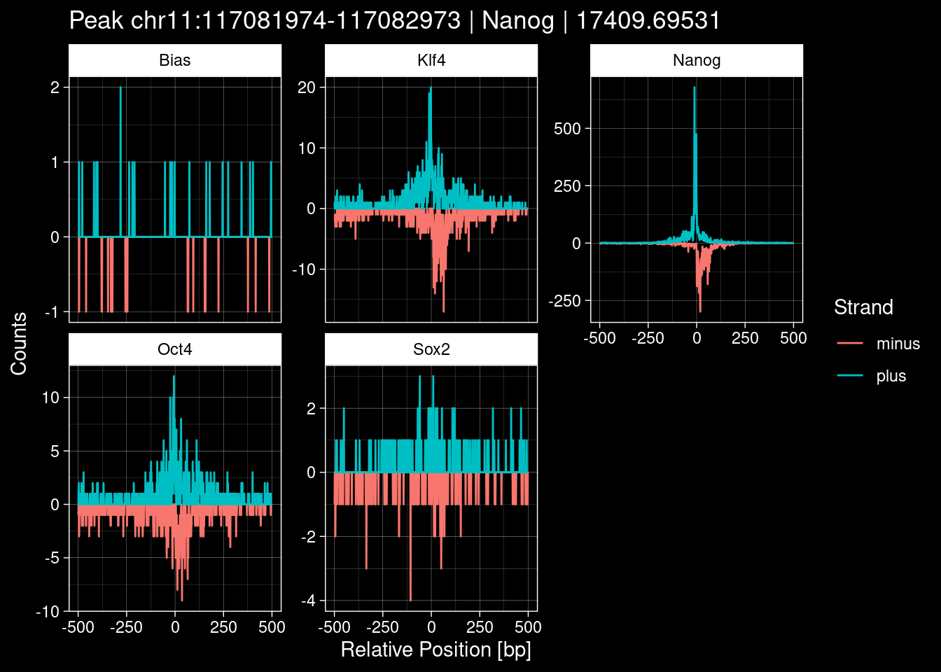
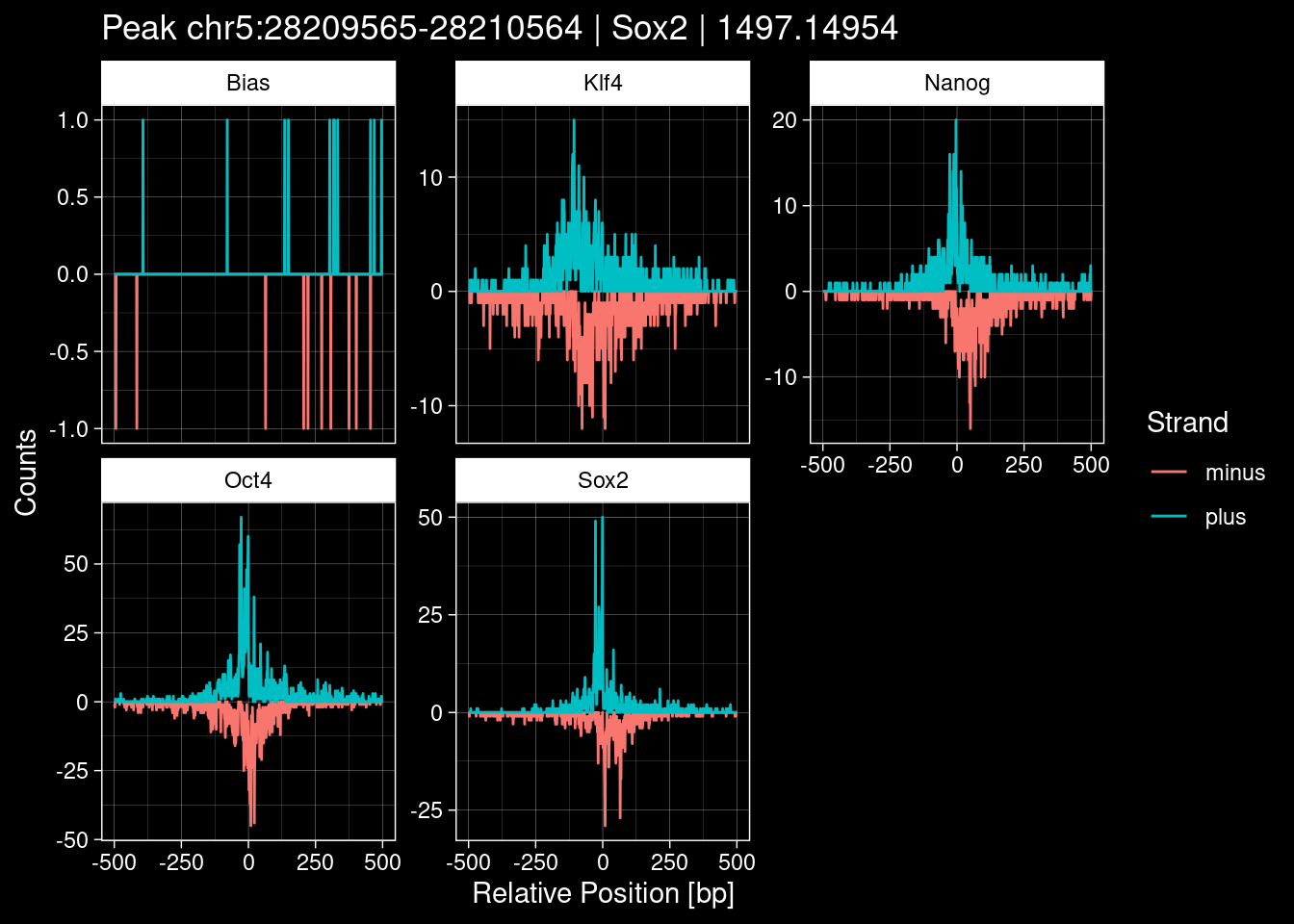
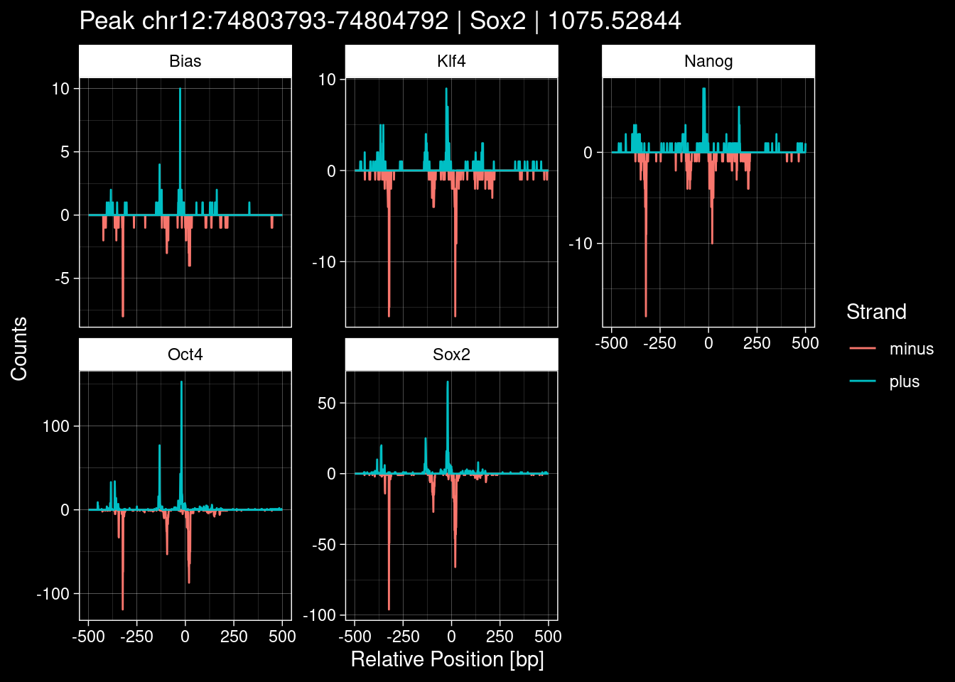
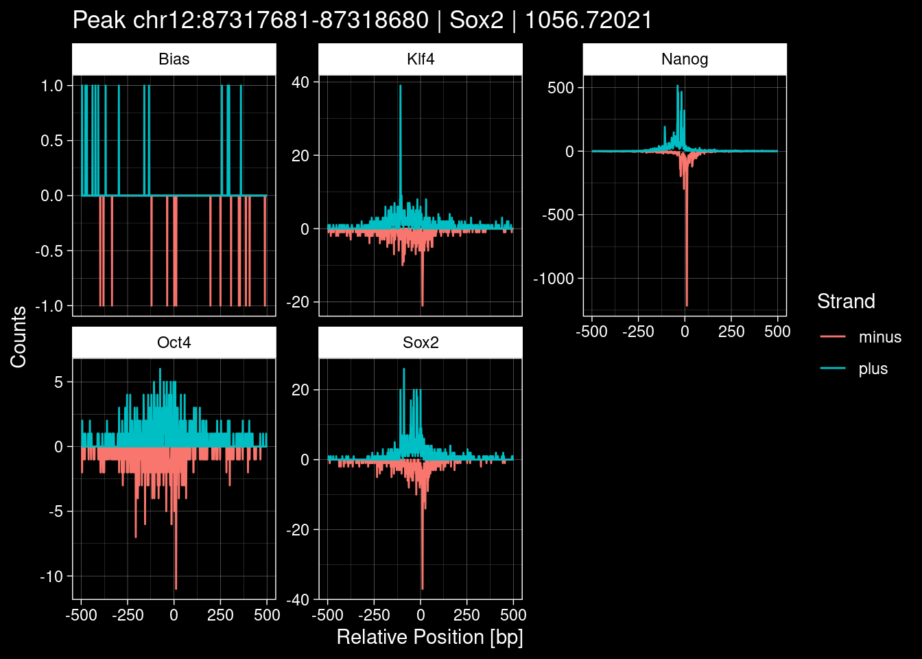
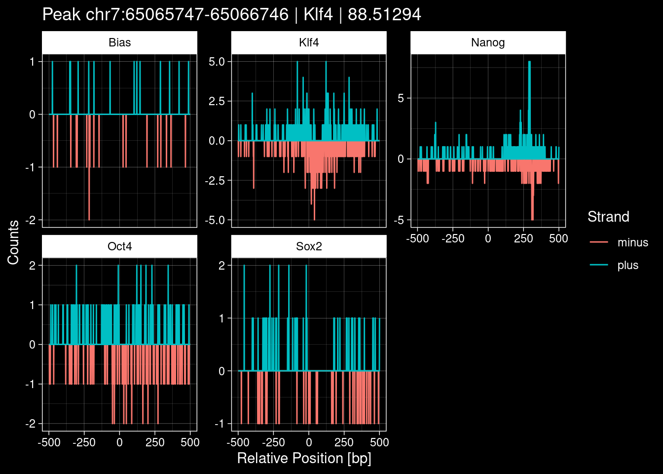
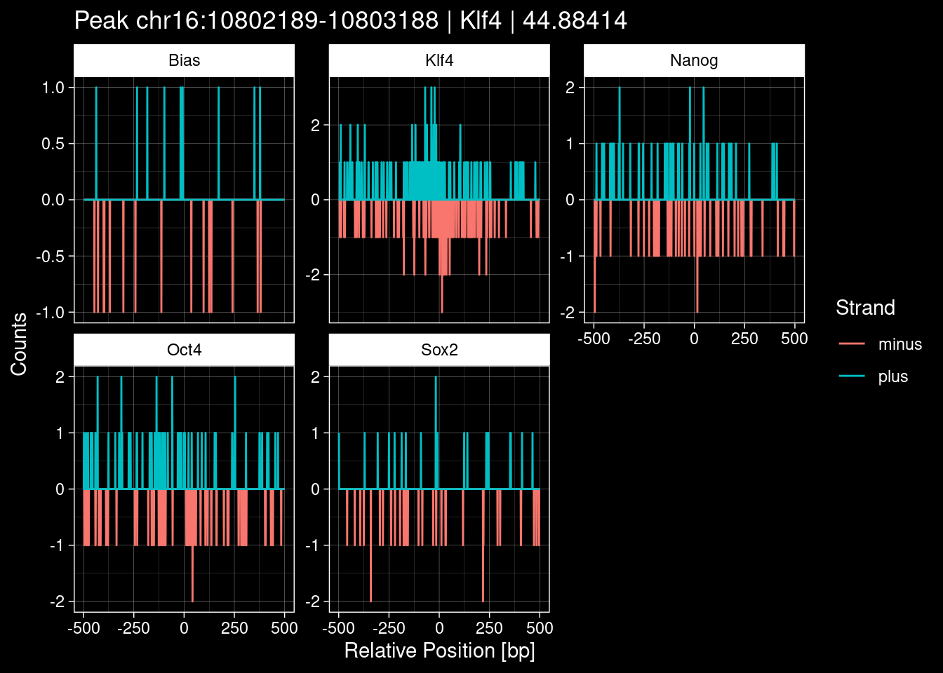
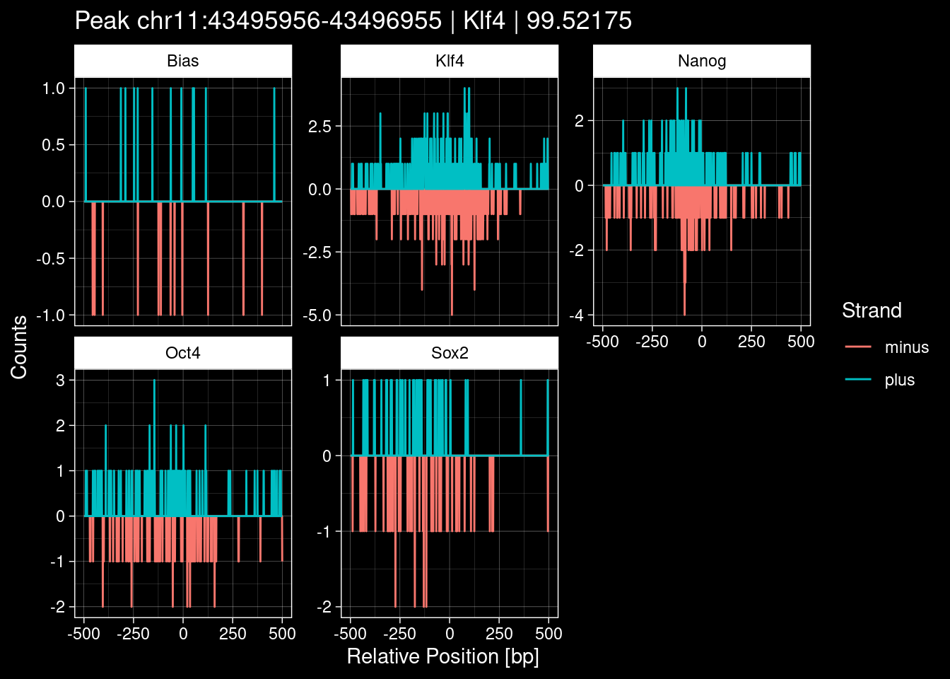
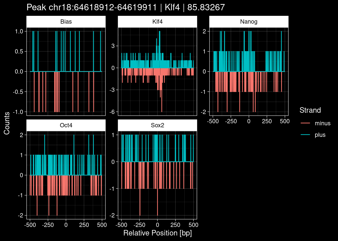
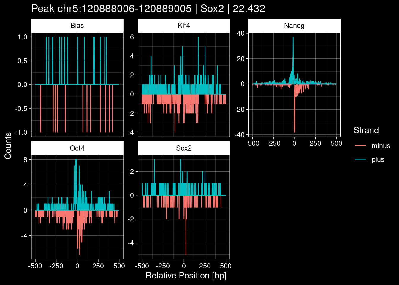
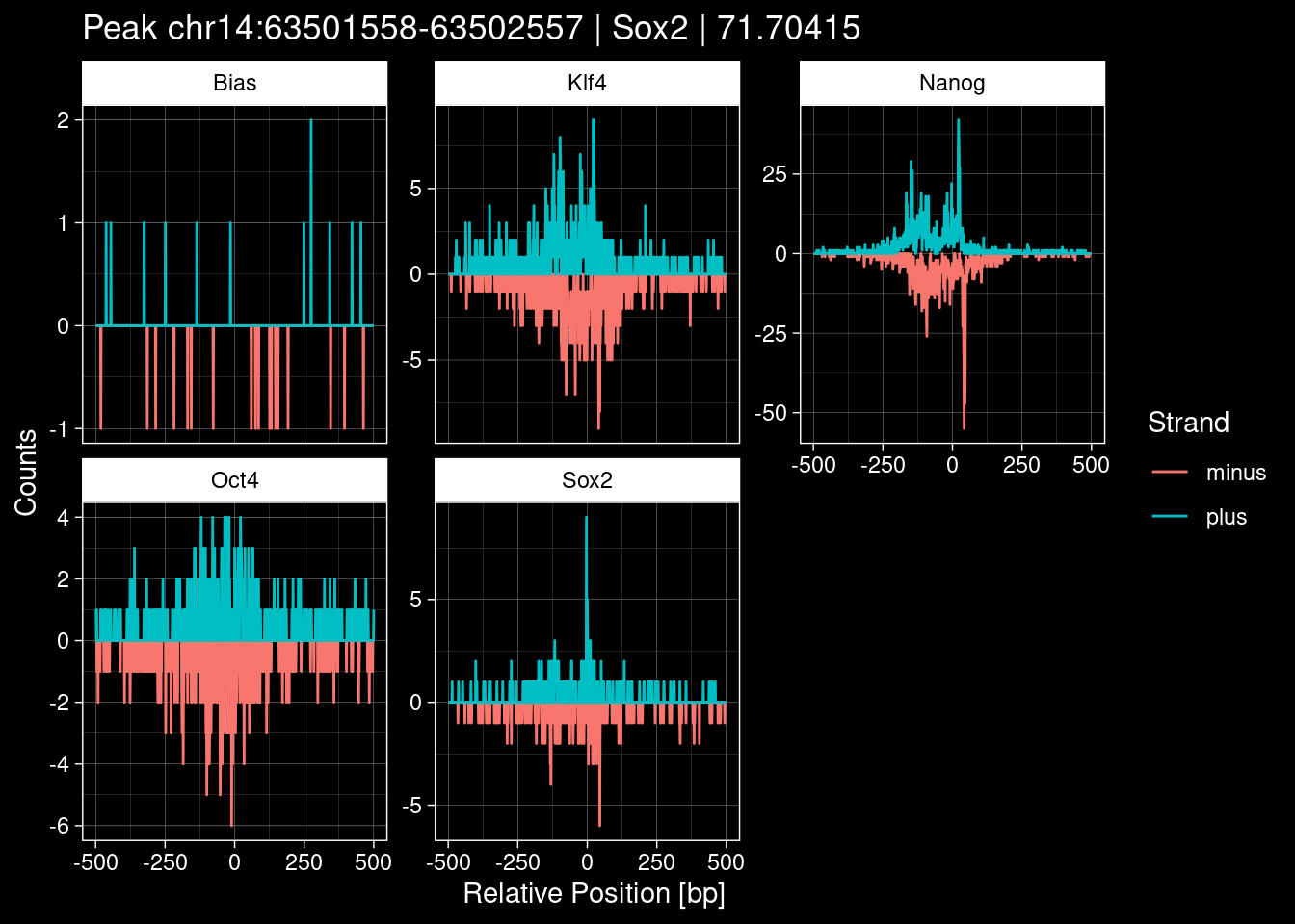
-> /home/philipp/BPNet/input/Nanog/train_counts.npy7.1 Examples: Highest Scoring Peaks
Click to expand
test_df <- peak_infos %>%
  as.data.frame() %>%
  dplyr::filter(set=="train") %>%
  dplyr::mutate(Region = paste0(seqnames, ":", start, "-", end)) %>%
  dplyr::group_by(TF) %>%
  slice_max(order_by=qValue, n=5) %>%
  select(Region, TF, qValue)

purrr::walk(1:nrow(test_df), function(i) {
  test_instance <- unlist(test_df[i, ])
  purrr::map_dfr(TFs, function(tf){
  tibble::tibble(position=-499:500,
                 plus = tf_counts[[tf]]$train$pos[match(test_instance["Region"], seq_names$train), ],
                 minus = -tf_counts[[tf]]$train$neg[match(test_instance["Region"], seq_names$train), ]) %>%
    dplyr::mutate(TF = tf, p_name = test_instance["Region"])
  }) %>%
  pivot_longer(cols=c(minus, plus)) %>%
  ggplot() +
  geom_line(aes(x=position, y=value, color=name)) +
  facet_wrap(~TF, scales="free_y") +
  ggdark::dark_theme_linedraw() +
  labs(x="Relative Position [bp]", y="Counts", color="Strand",
       title=paste0("Peak ", test_instance["Region"], " | ", test_instance["TF"],
                    " | ", test_instance["qValue"])) -> p
  print(p)
})
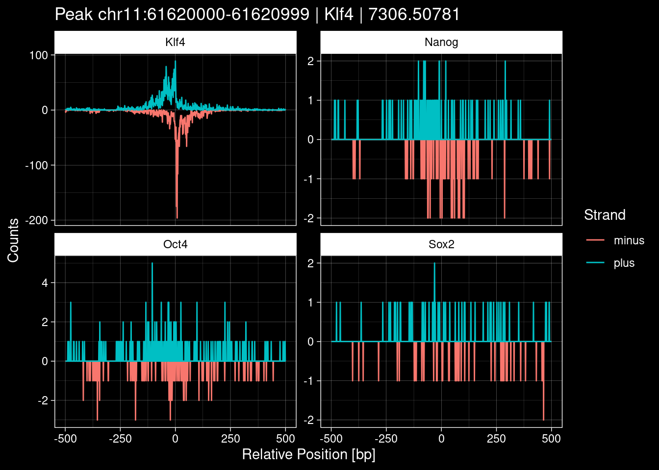
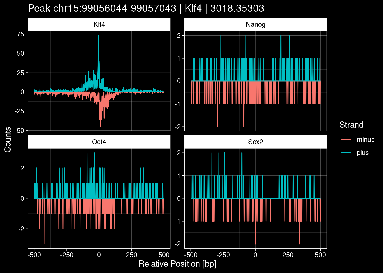
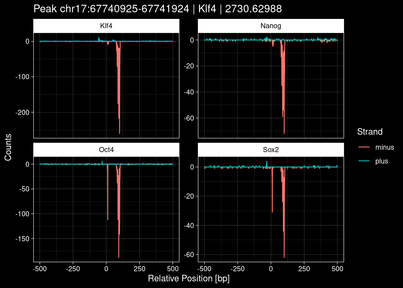


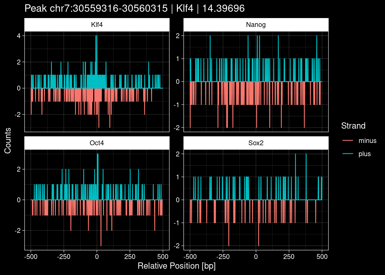
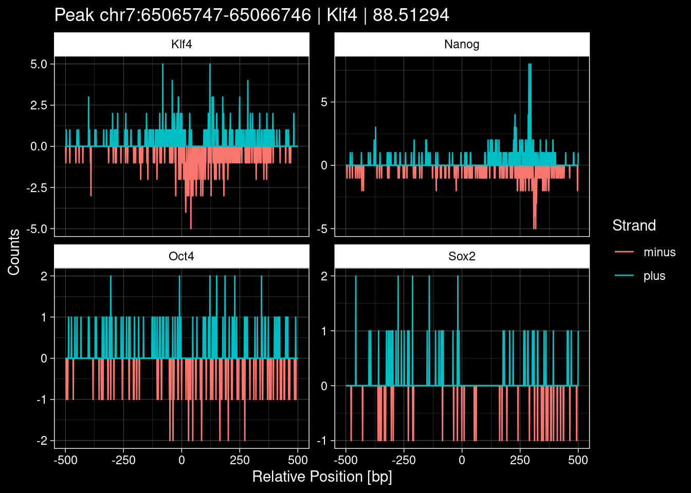
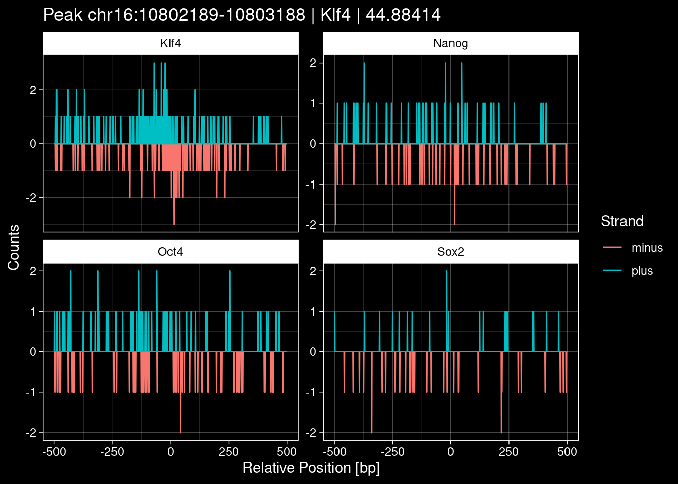
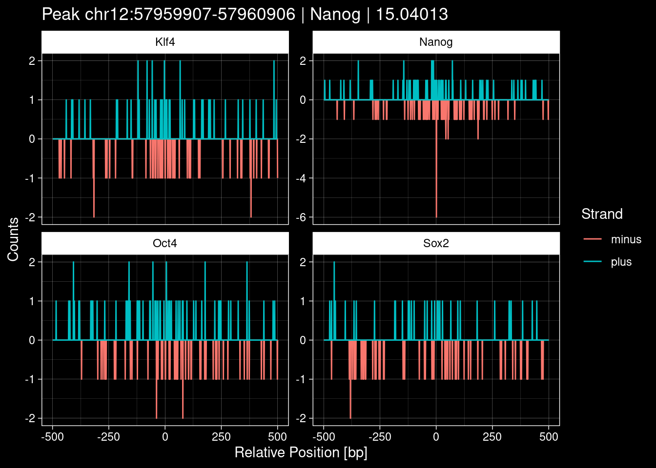
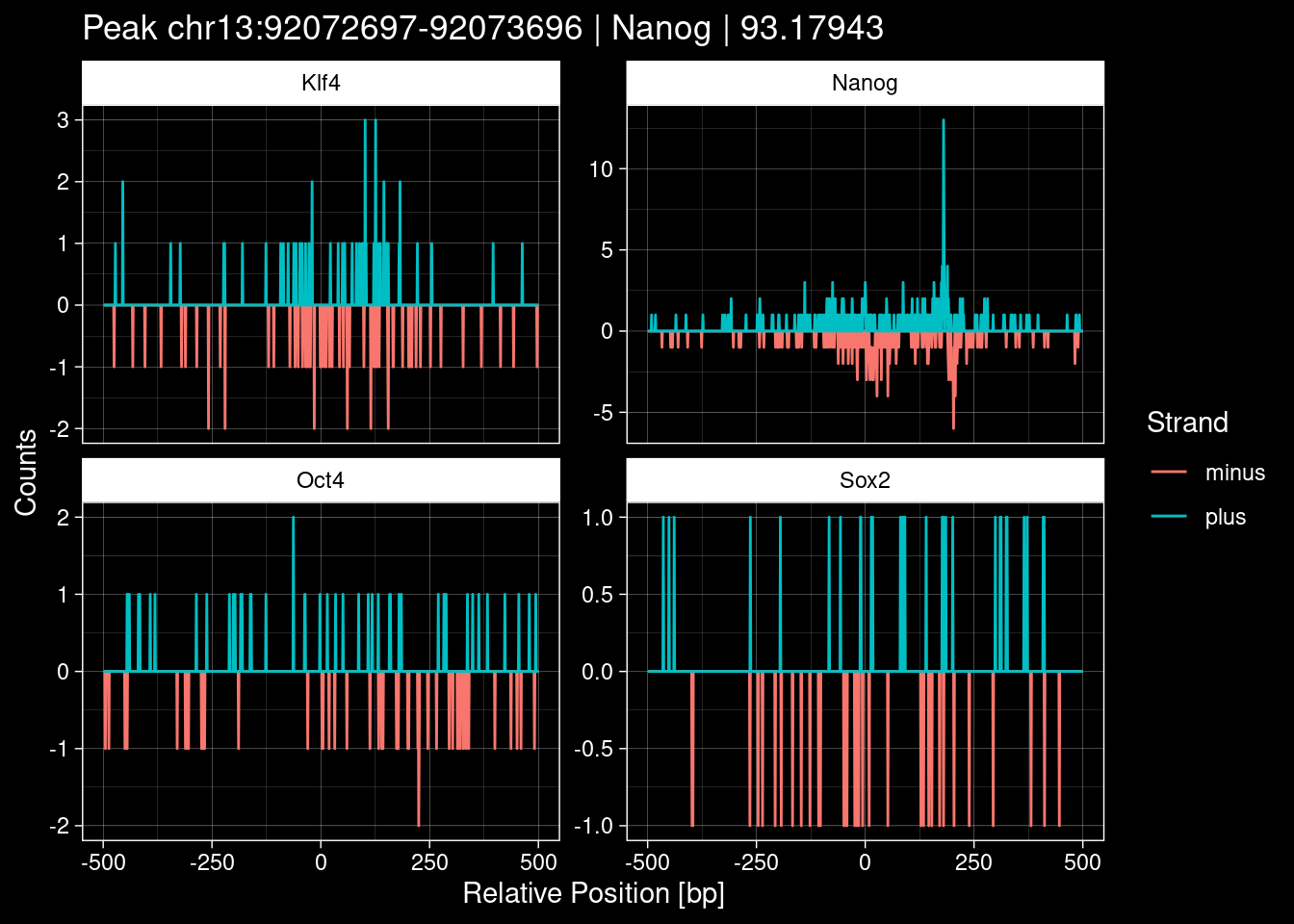
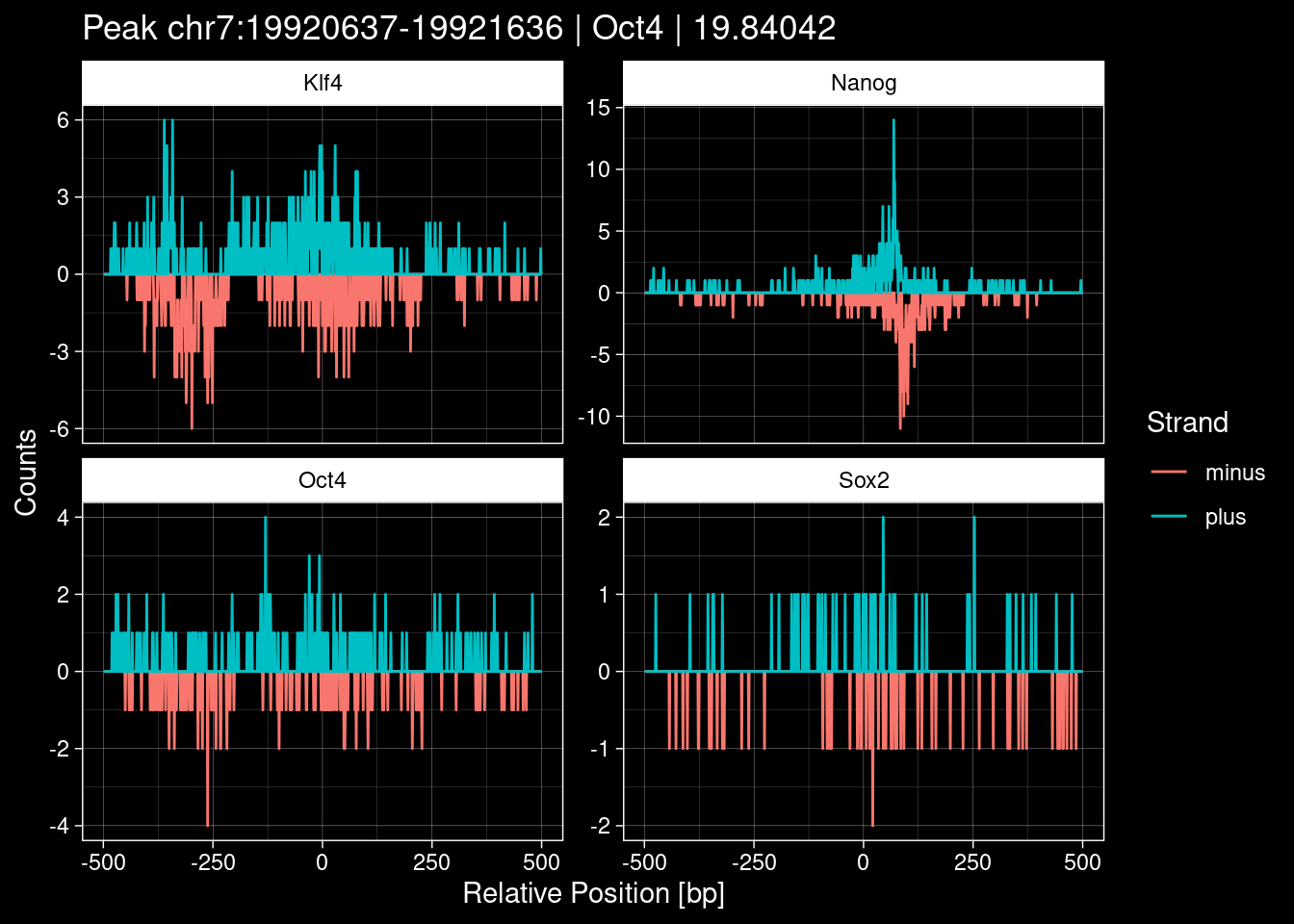
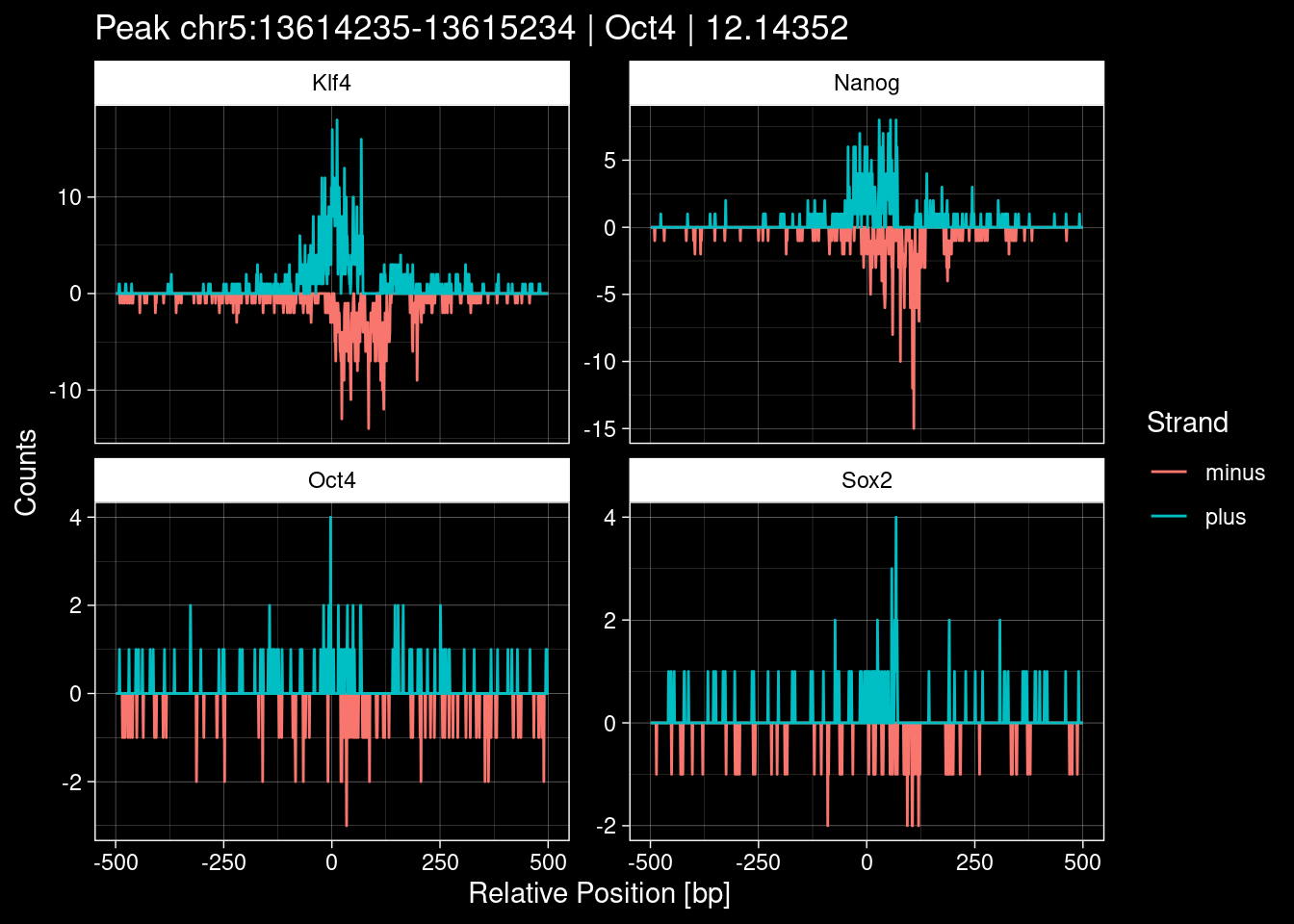
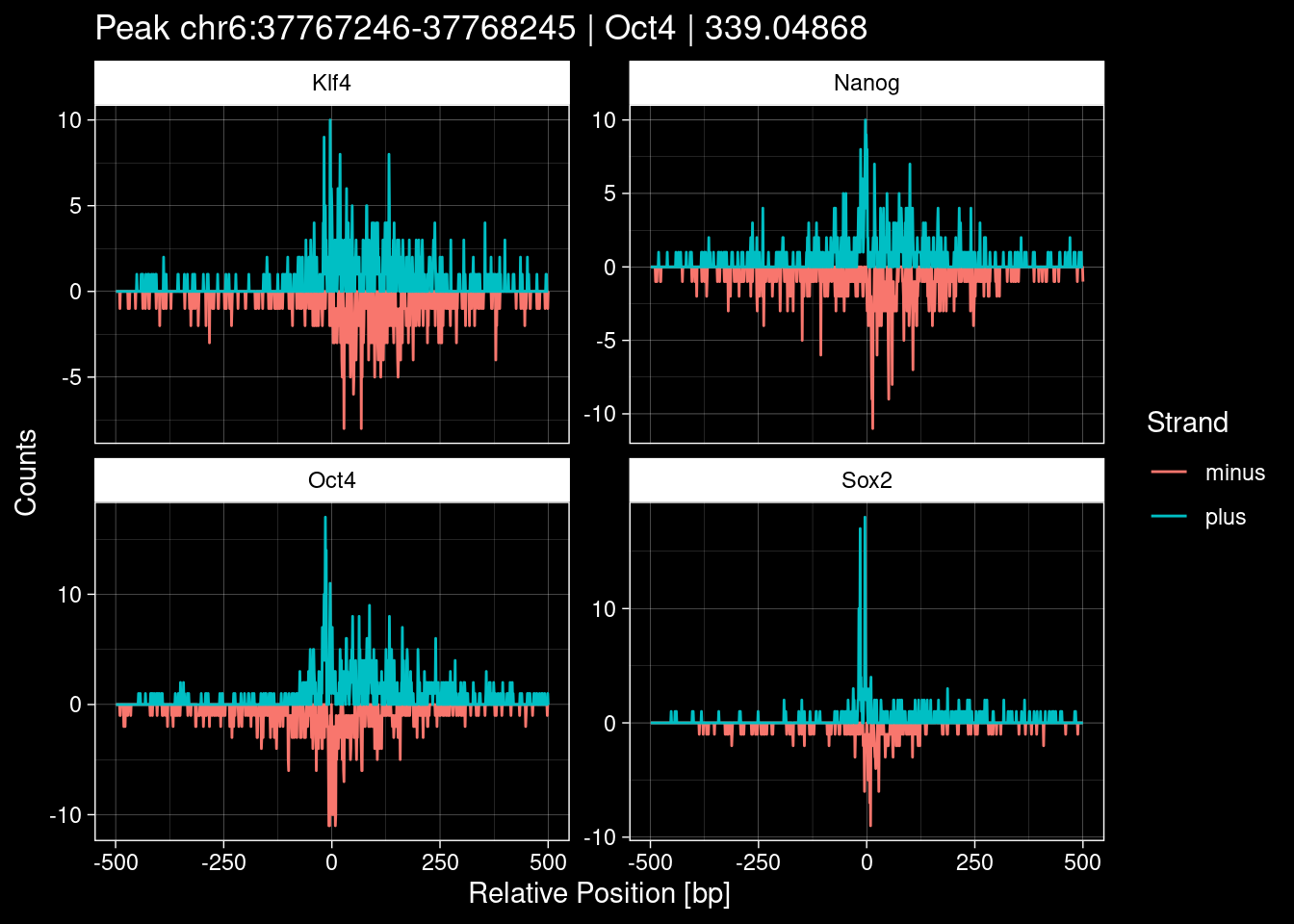
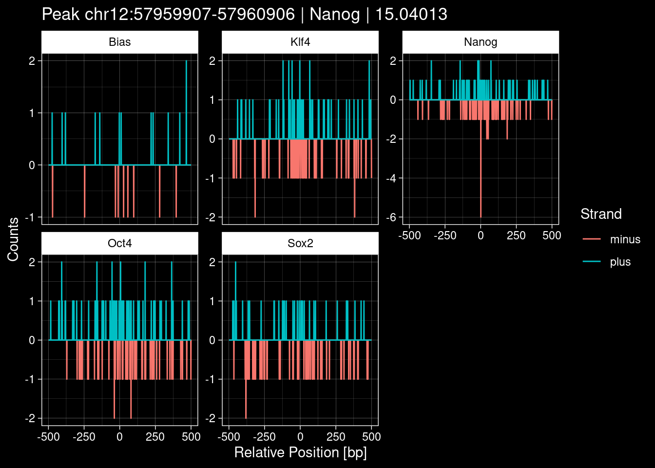
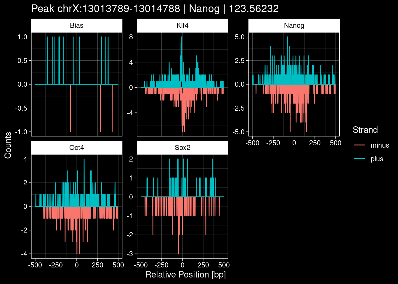
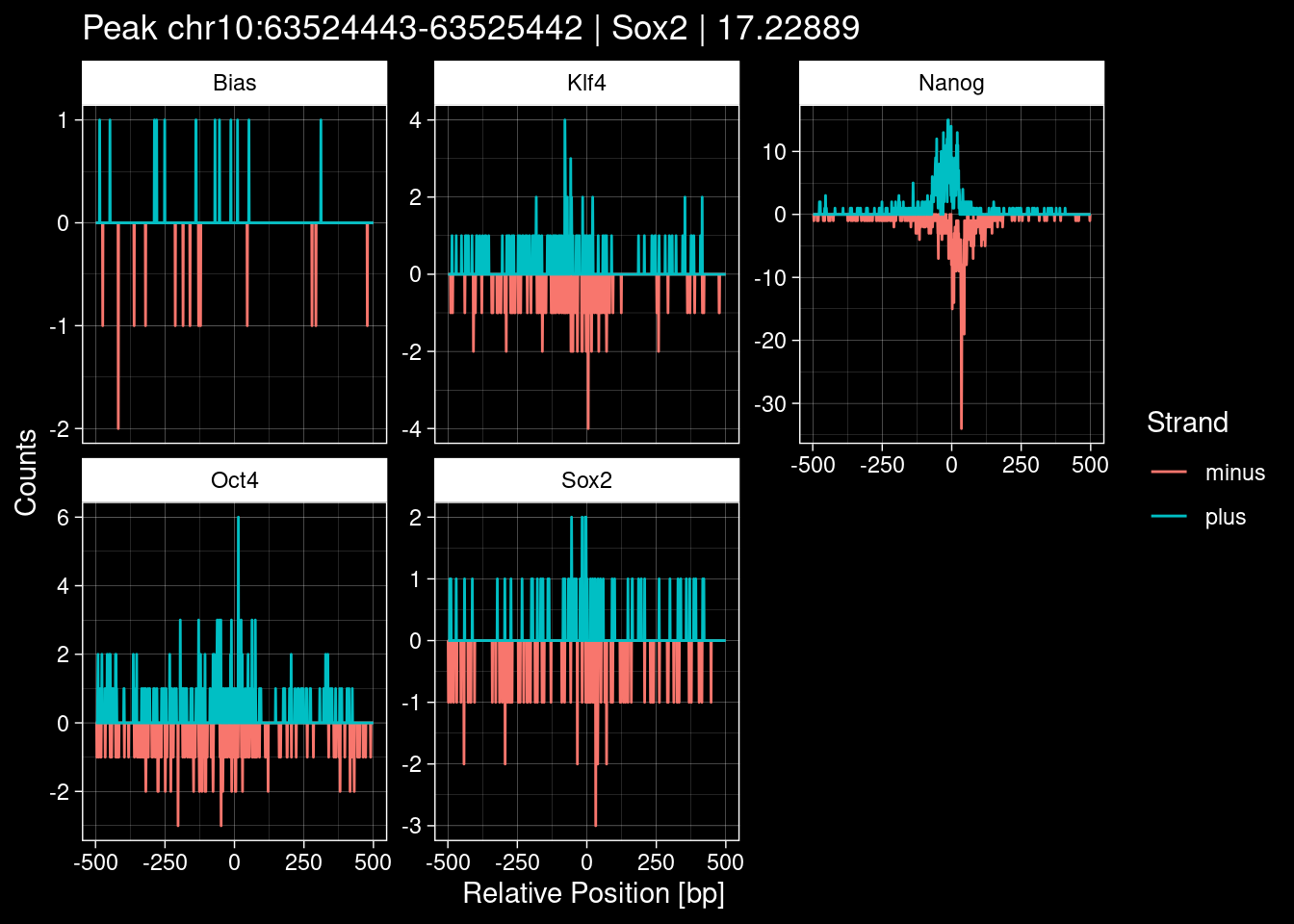
7.2 Examples: Random Peaks
Click to expand
set.seed(42)
test_df <- peak_infos %>%
  as.data.frame() %>%
  dplyr::filter(set=="train") %>%
  dplyr::mutate(Region = paste0(seqnames, ":", start, "-", end)) %>%
  dplyr::group_by(TF) %>%
  slice_sample(n=5) %>%
  select(Region, TF, qValue)

purrr::walk(1:nrow(test_df), function(i) {
  test_instance <- unlist(test_df[i, ])
  purrr::map_dfr(TFs, function(tf){
  tibble::tibble(position=-499:500,
                 plus = tf_counts[[tf]]$train$pos[match(test_instance["Region"], seq_names$train), ],
                 minus = -tf_counts[[tf]]$train$neg[match(test_instance["Region"], seq_names$train), ]) %>%
    dplyr::mutate(TF = tf, p_name = test_instance["Region"])
  }) %>%
  pivot_longer(cols=c(minus, plus)) %>%
  ggplot() +
  geom_line(aes(x=position, y=value, color=name)) +
  facet_wrap(~TF, scales="free_y") +
  ggdark::dark_theme_linedraw() +
  labs(x="Relative Position [bp]", y="Counts", color="Strand",
       title=paste0("Peak ", test_instance["Region"], " | ", test_instance["TF"],
                    " | ", test_instance["qValue"])) -> p
  print(p)
})
8 Extract the Control (Patchcap) Counts
patchcap_input <-
  c("pos", "neg") %>%
  purrr::set_names() %>%
  purrr::map(function(strand){
  rtracklayer::import.bw(paste0("../data/chip-nexus/patchcap/counts.", strand, ".bw")) %>%
    GenomicRanges::coverage(., weight = "score")
})

ctrl_counts <- furrr::future_imap(chrom_list, function(set_chroms, set_name) {

  peak_info_subset <- peak_infos[seqnames(peak_infos) %in% set_chroms]

  c("pos", "neg") %>%
    purrr::set_names() %>%
    purrr::map(function(strand) {

      mtx <- matrix(data=0, ncol=peak_width, nrow=length(peak_info_subset))

      for (seq_index in 1:nrow(mtx)) {
        chrom_index <- as.character(peak_info_subset[seq_index]@seqnames)
        position_index <- peak_info_subset[seq_index]@ranges@start:(peak_info_subset[seq_index]@ranges@start+peak_width-1)
        mtx[seq_index, ] = as.numeric(patchcap_input[[strand]][[chrom_index]][position_index])
      }
      mtx
  })
})str(ctrl_counts)List of 3
$ tune :List of 2
..$ pos: num [1:29277, 1:1000] 0 0 0 0 0 0 0 0 0 0 ...
..$ neg: num [1:29277, 1:1000] 0 0 0 0 0 0 0 0 0 0 ...
$ test :List of 2
..$ pos: num [1:27727, 1:1000] 0 0 0 0 0 0 0 0 0 0 ...
..$ neg: num [1:27727, 1:1000] 0 0 0 0 0 0 0 0 0 0 ...
$ train:List of 2
..$ pos: num [1:93904, 1:1000] 0 0 0 0 0 0 0 0 1 0 ...
..$ neg: num [1:93904, 1:1000] 0 0 0 0 0 0 0 0 0 0 ...Write the matrices in binary format to disk using reticulate
import numpy as np

for set_name, set_entry in r.ctrl_counts.items():
  mtx = np.stack([set_entry["pos"], set_entry["neg"]], axis=1).astype(np.float32)
  print(f"\t{set_name} shape: {mtx.shape}")
  save_path = f"{r.output_dir}patchcap/{set_name}_counts.npy"
  print(f"\t-> {save_path}")
  np.save(file=save_path, arr=mtx)
tune shape: (29277, 2, 1000)
-> /home/philipp/BPNet/input/patchcap/tune_counts.npy
test shape: (27727, 2, 1000)
-> /home/philipp/BPNet/input/patchcap/test_counts.npy
train shape: (93904, 2, 1000)
-> /home/philipp/BPNet/input/patchcap/train_counts.npy8.1 Examples: Highest Scoring Peaks with Bias
test_instance <- peak_infos %>%
  as.data.frame() %>%
  dplyr::filter(set=="test") %>%
  dplyr::filter(seqnames=="chr1", start >= 180924752-1000, end <= 180925152+1000) %>%
  dplyr::mutate(Region = paste0(seqnames, ":", start, "-", end)) %>%
  dplyr::select(Region, TF, qValue) %>%
  .[1, ]
print(test_instance)
Region TF qValue
1 chr1:180924435-180925434 Sox2 436.0653p <- purrr::map_dfr(TFs, function(tf){
tibble::tibble(position=-499:500,
plus = tf_counts[[tf]]$test$pos[match(test_instance["Region"], seq_names$test), ],
minus = -tf_counts[[tf]]$test$neg[match(test_instance["Region"], seq_names$test), ]) %>%
dplyr::mutate(TF = tf, p_name = test_instance["Region"])
}) %>%
rbind(
tibble::tibble(position=-499:500,
plus = ctrl_counts$test$pos[match(test_instance["Region"], seq_names$test), ],
minus = -ctrl_counts$test$neg[match(test_instance["Region"], seq_names$test), ],
TF = "patchcap", p_name = test_instance["Region"])
) %>%
pivot_longer(cols=c(minus, plus)) %>%
dplyr::mutate(TF = factor(TF, levels=names(colors))) %>%
ggplot() +
geom_line(aes(x=position, y=value, color=TF, alpha=name), size=0.2) +
facet_wrap(~TF, ncol=1, scales="free_y") +
labs(x="Relative Position [bp]", y="Counts", color="Strand",
title=test_instance["Region"]) +
#scale_color_manual(values=c("minus"="darkred", "plus"="forestgreen")) +
scale_color_manual(values=colors) +
scale_alpha_manual(values=c("plus" = 1, "minus" = 1)) +
theme_bw() +
theme(plot.title = element_text(size=10, hjust=0.5), strip.background = element_rect(fill=NA))
ggsave(filename = "/home/philipp/BPNet/out/figures/example_high_q.pdf",
plot = p, width = 4, height = 8)
p +
ggdark::dark_theme_linedraw()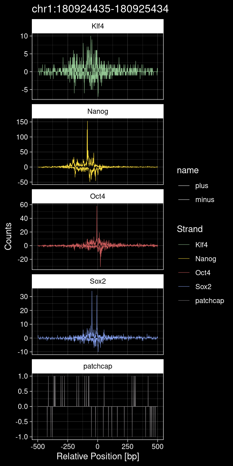
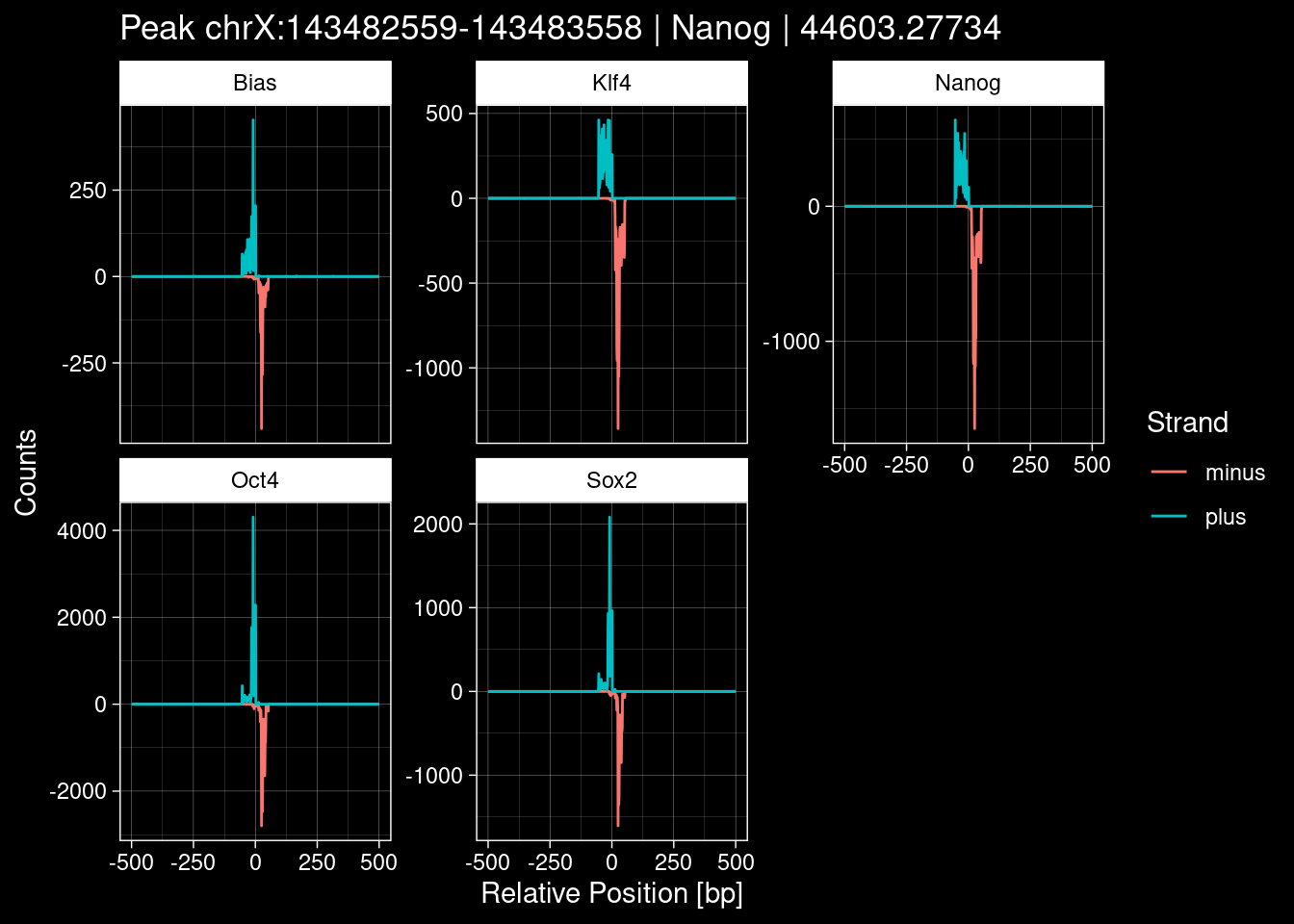
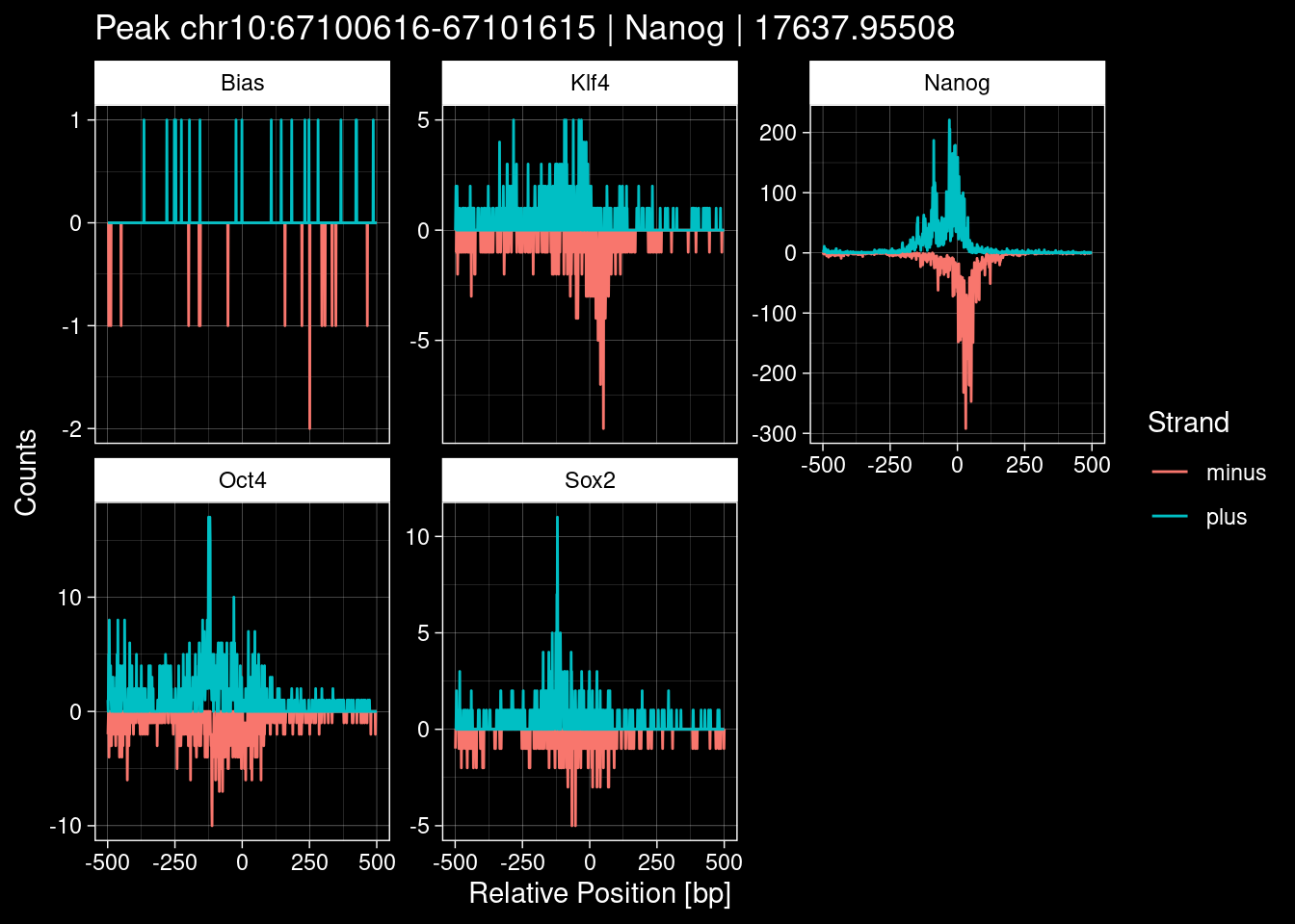
Click to view more plots
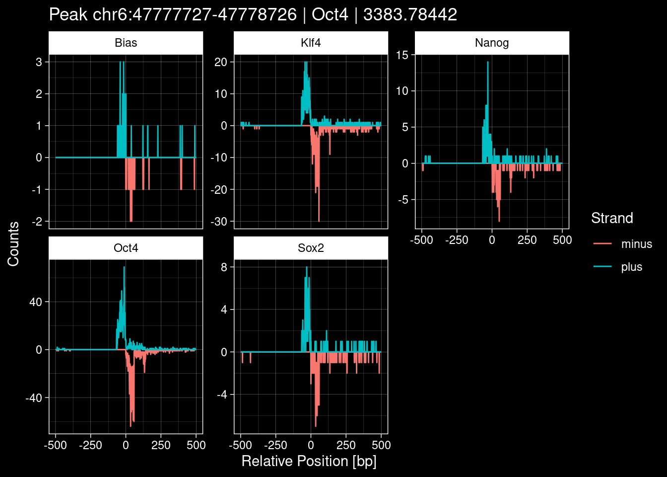
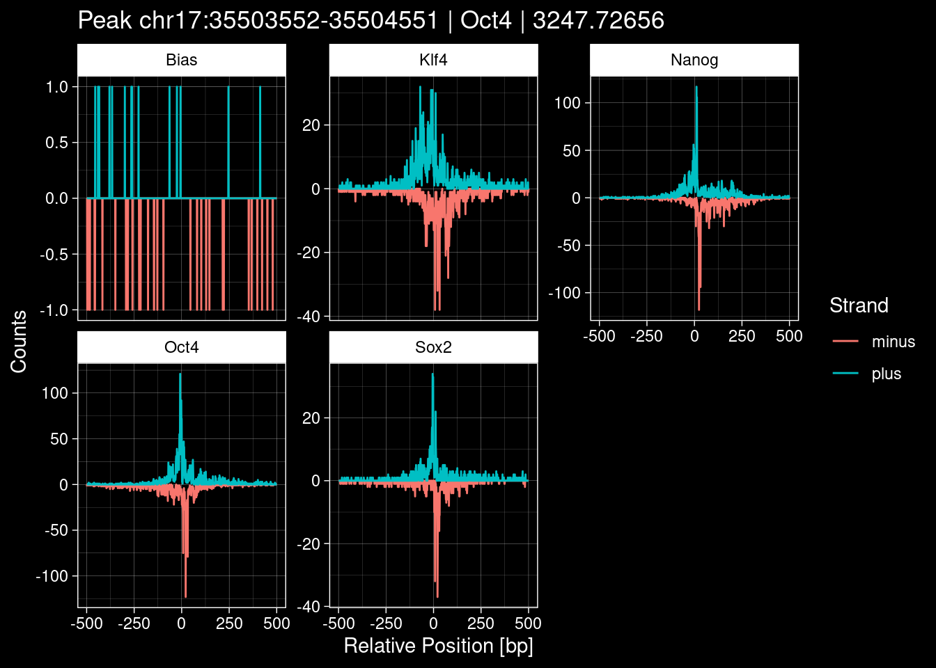
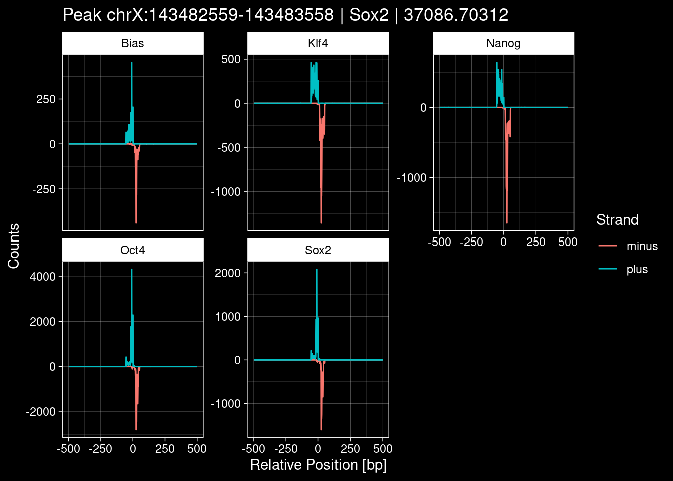
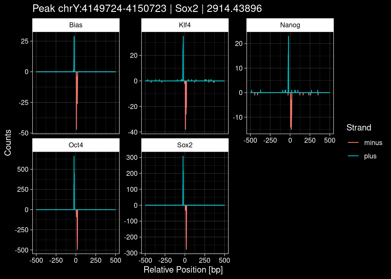
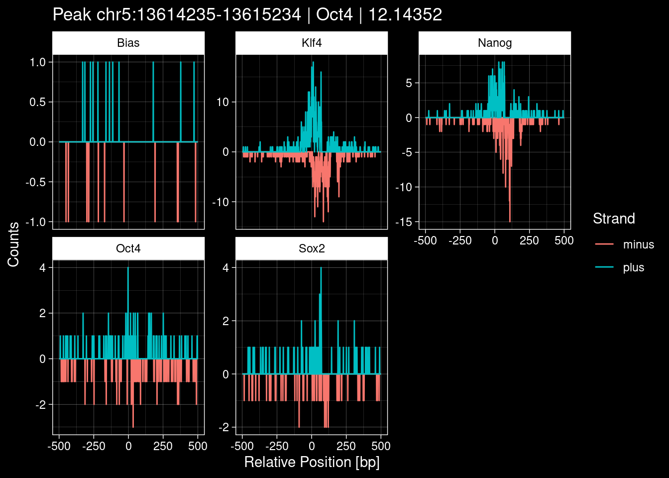
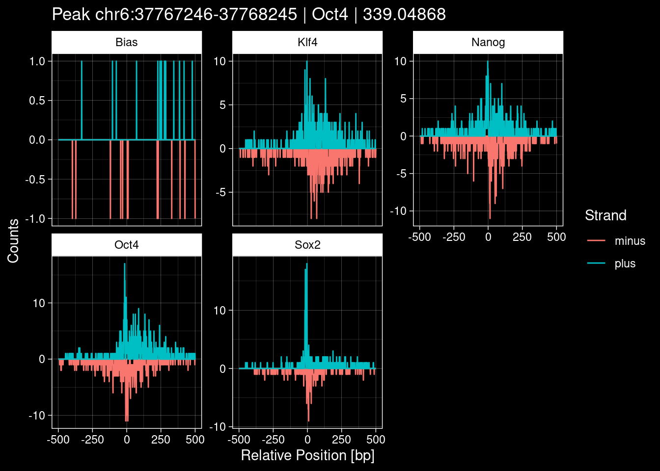
test_df <- peak_infos %>%
as.data.frame() %>%
dplyr::filter(set=="train") %>%
dplyr::mutate(Region = paste0(seqnames, ":", start, "-", end)) %>%
dplyr::group_by(TF) %>%
slice_max(order_by=qValue, n=5) %>%
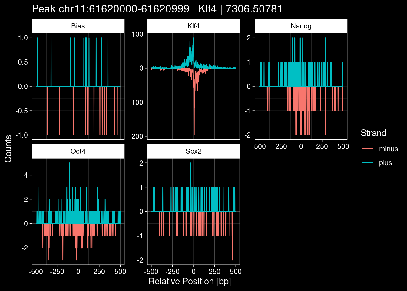
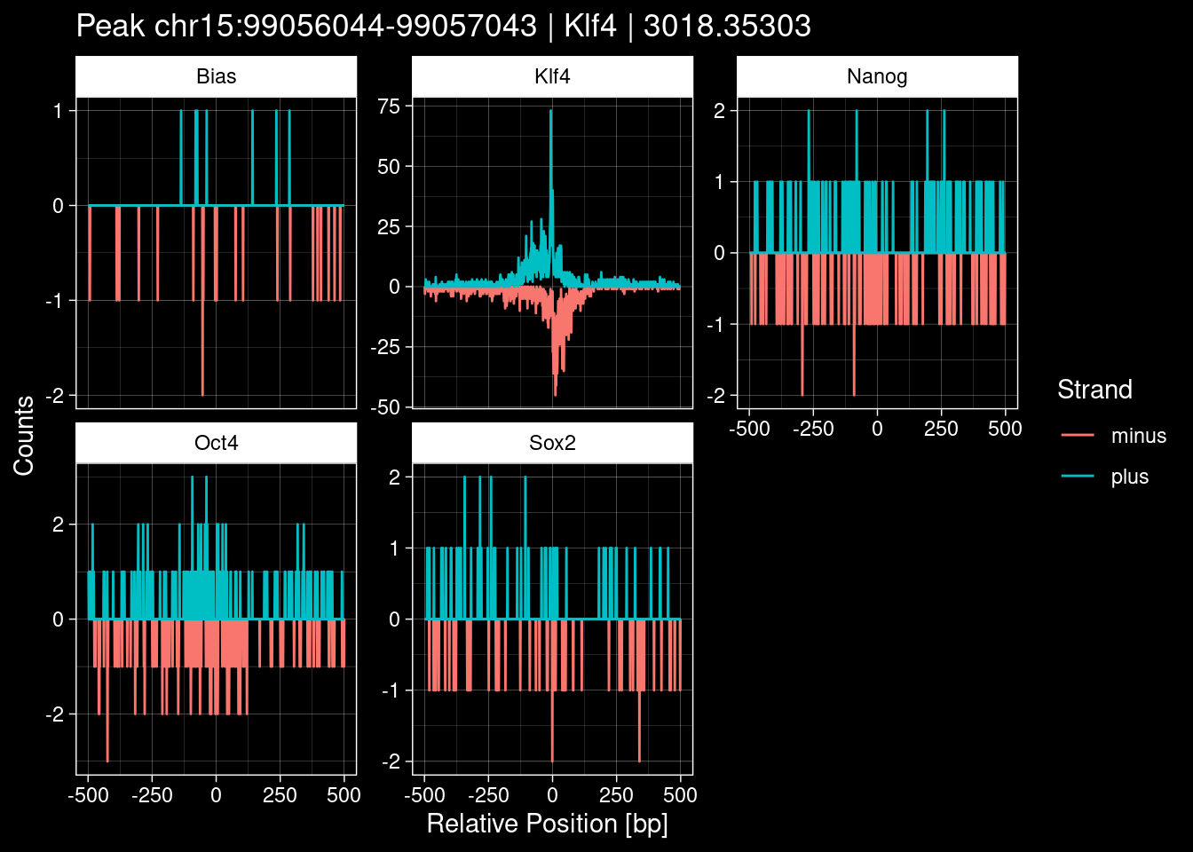
select(Region, TF, qValue)
purrr::walk(1:nrow(test_df), function(i) {
test_instance <- unlist(test_df[i, ])
purrr::map_dfr(TFs, function(tf){
tibble::tibble(position=-499:500,
plus = tf_counts[[tf]]$train$pos[match(test_instance["Region"], seq_names$train), ],
minus = -tf_counts[[tf]]$train$neg[match(test_instance["Region"], seq_names$train), ]) %>%
dplyr::mutate(TF = tf, p_name = test_instance["Region"])
}) %>%
rbind(
tibble::tibble(position=-499:500,
plus = ctrl_counts$train$pos[match(test_instance["Region"], seq_names$train), ],
minus = -ctrl_counts$train$neg[match(test_instance["Region"], seq_names$train), ],
TF = "Bias", p_name = test_instance["Region"])
) %>%
pivot_longer(cols=c(minus, plus)) %>%
ggplot() +
geom_line(aes(x=position, y=value, color=name)) +
facet_wrap(~TF, scales="free_y") +
ggdark::dark_theme_linedraw() +
labs(x="Relative Position [bp]", y="Counts", color="Strand",
title=paste0("Peak ", test_instance["Region"], " | ", test_instance["TF"],
" | ", test_instance["qValue"])) -> p
print(p)
})


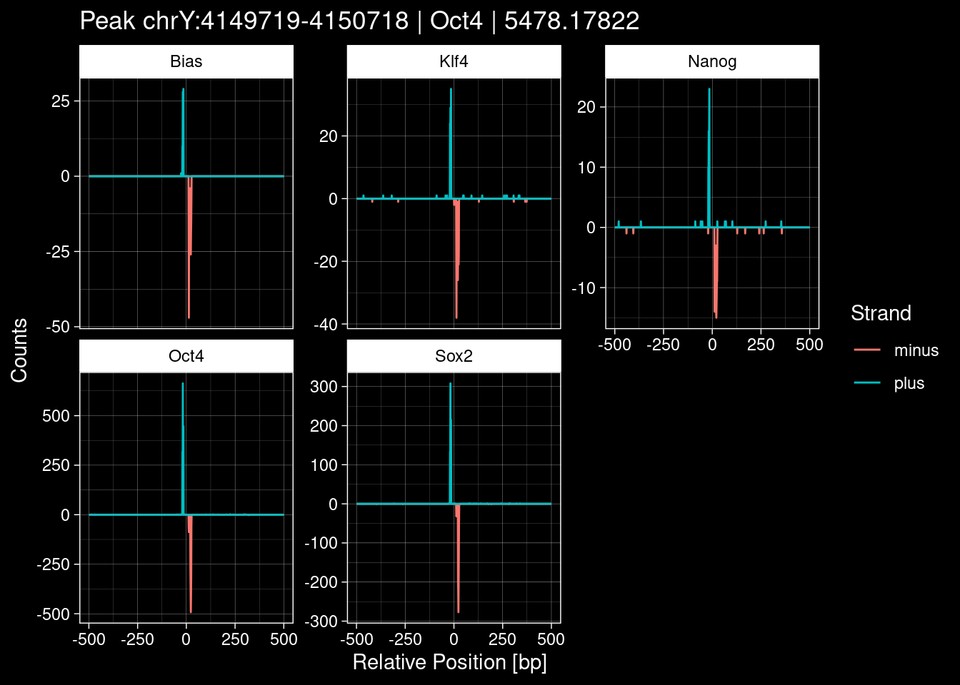
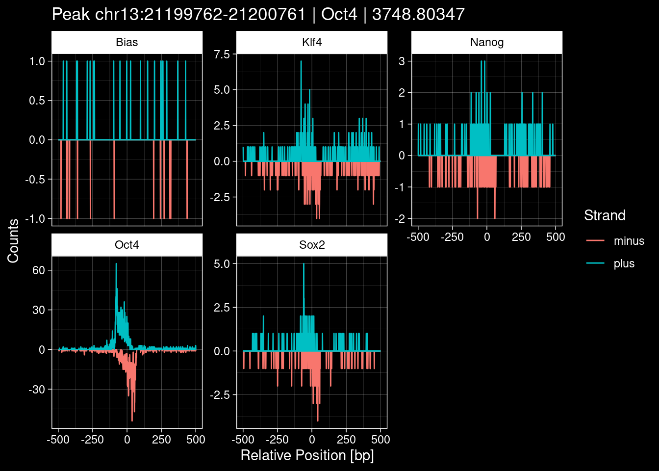
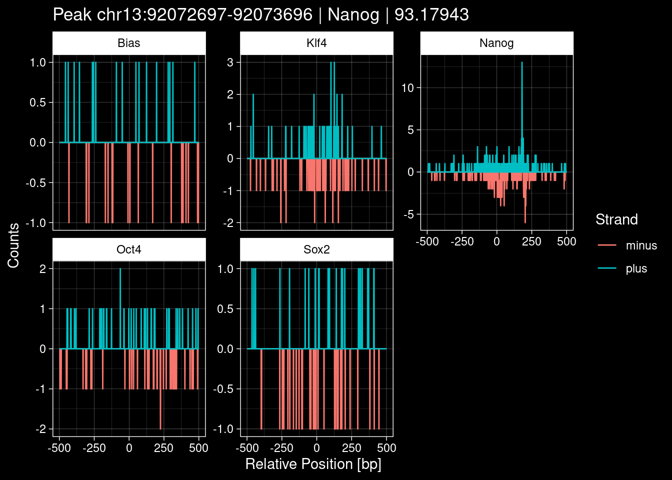
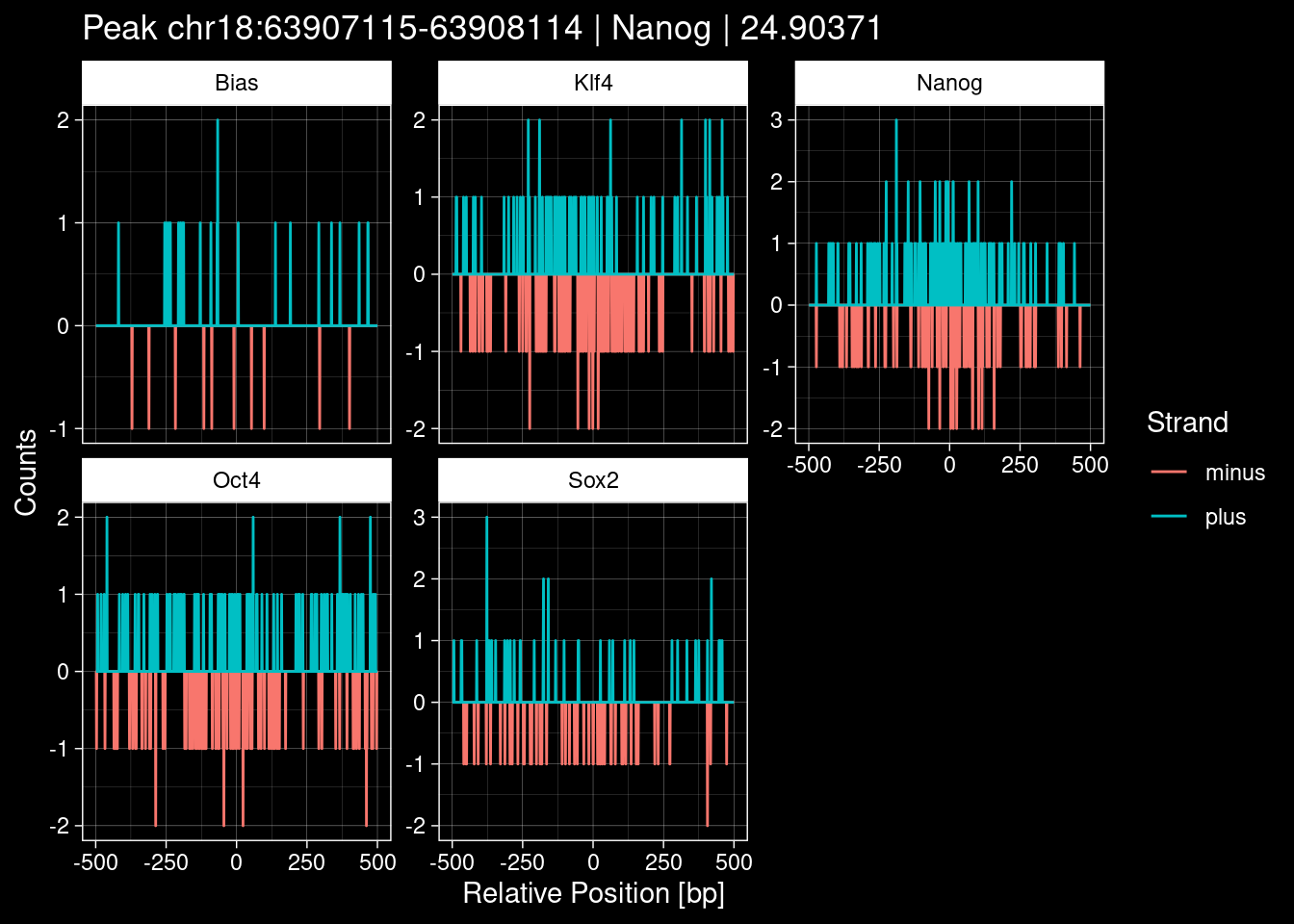
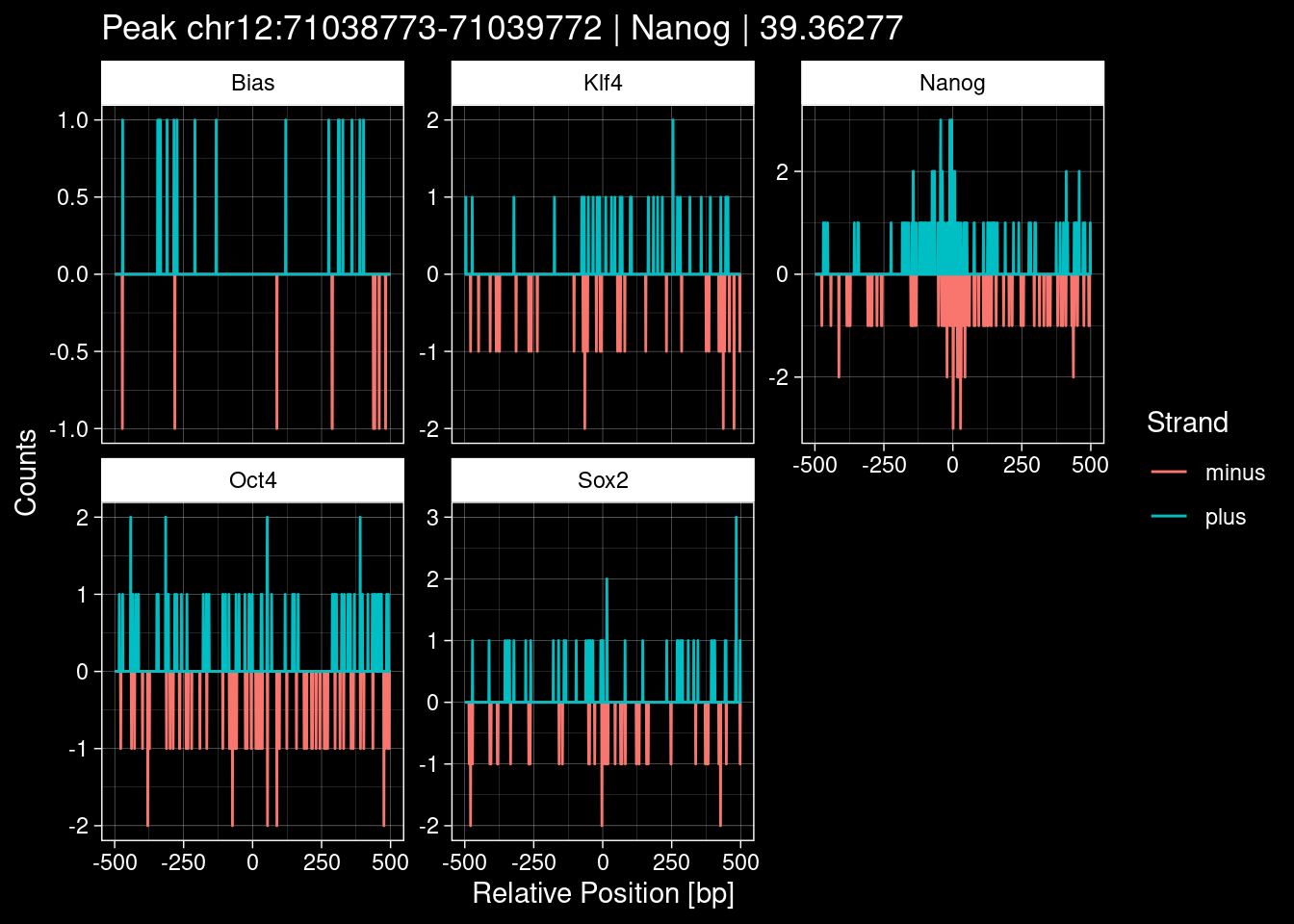
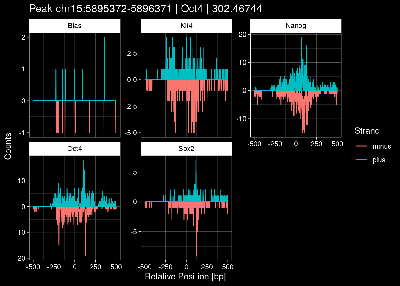
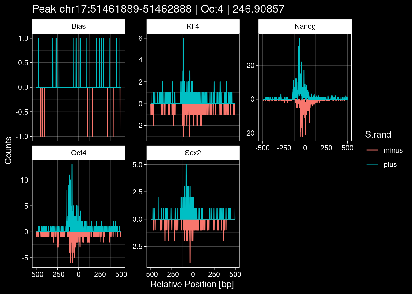
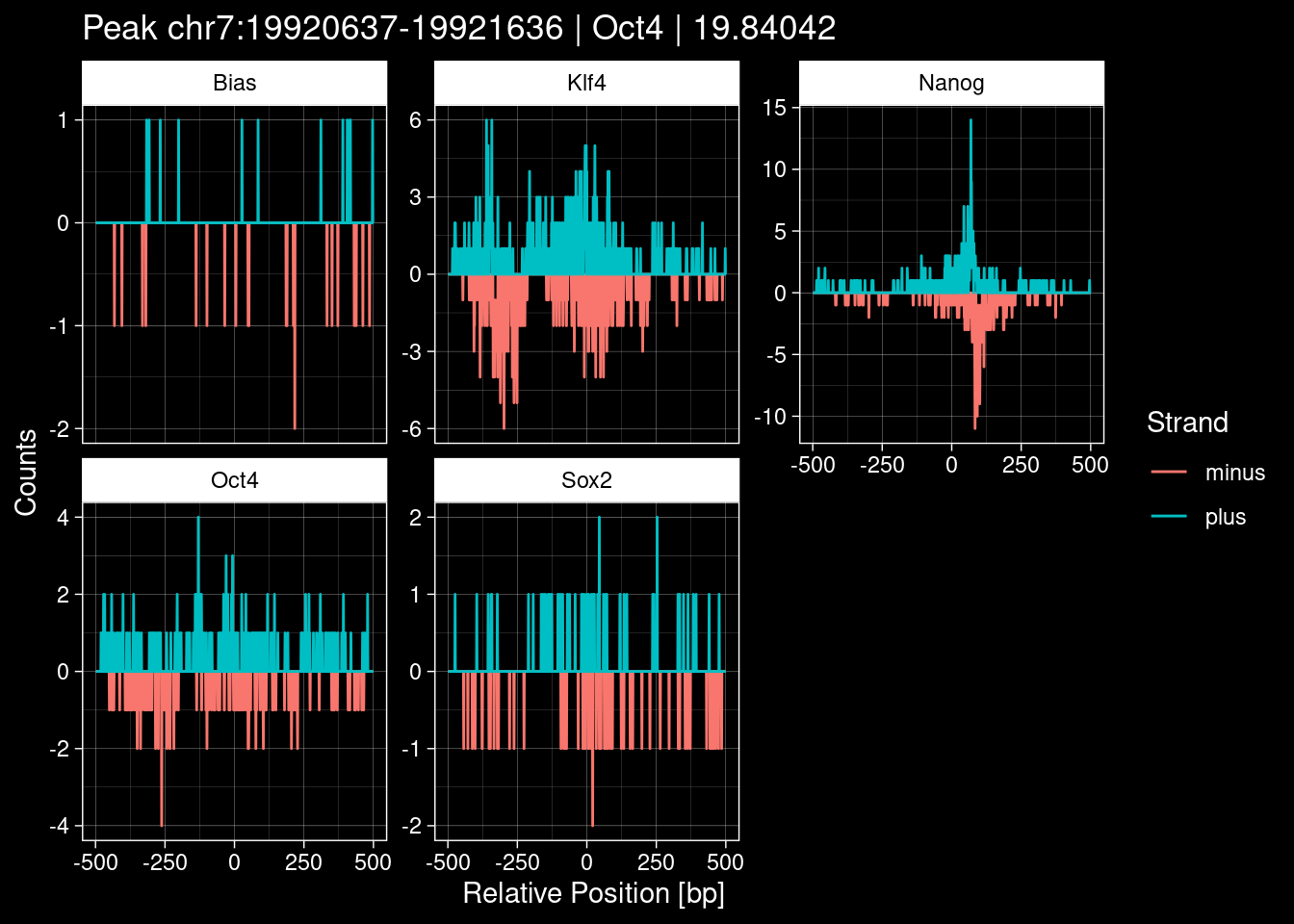
8.2 Examples: Random Peaks with Bias
test_instance <- peak_infos %>%
  as.data.frame() %>%
  dplyr::filter(set=="test") %>%
  dplyr::filter(seqnames=="chr1", start >= 4000, end <= 100000000) %>%
  dplyr::mutate(Region = paste0(seqnames, ":", start, "-", end)) %>%
  dplyr::select(Region, TF, qValue) %>%
  .[1000, ]
print(test_instance)
Region TF qValue
1000 chr1:58392603-58393602 Oct4 21.10429p <- purrr::map_dfr(TFs, function(tf){
tibble::tibble(position=-499:500,
plus = tf_counts[[tf]]$test$pos[match(test_instance["Region"], seq_names$test), ],
minus = -tf_counts[[tf]]$test$neg[match(test_instance["Region"], seq_names$test), ]) %>%
dplyr::mutate(TF = tf, p_name = test_instance["Region"])
}) %>%
rbind(
tibble::tibble(position=-499:500,
plus = ctrl_counts$test$pos[match(test_instance["Region"], seq_names$test), ],
minus = -ctrl_counts$test$neg[match(test_instance["Region"], seq_names$test), ],
TF = "patchcap", p_name = test_instance["Region"])
) %>%
pivot_longer(cols=c(minus, plus)) %>%
dplyr::mutate(TF = factor(TF, levels=names(colors))) %>%
ggplot() +
geom_line(aes(x=position, y=value, color=TF, alpha=name), size=0.2) +
facet_wrap(~TF, ncol=1, scales="free_y") +
labs(x="Relative Position [bp]", y="Counts", color="Strand",
title=test_instance["Region"]) +
#scale_color_manual(values=c("minus"="darkred", "plus"="forestgreen")) +
scale_color_manual(values=colors) +
scale_alpha_manual(values=c("plus" = 1, "minus" = 1)) +
theme_bw() +
theme(plot.title = element_text(size=10, hjust=0.5), strip.background = element_rect(fill=NA))
ggsave(filename = "/home/philipp/BPNet/out/figures/example_low_q.pdf",
plot = p, width = 4, height = 8)
p +
ggdark::dark_theme_linedraw()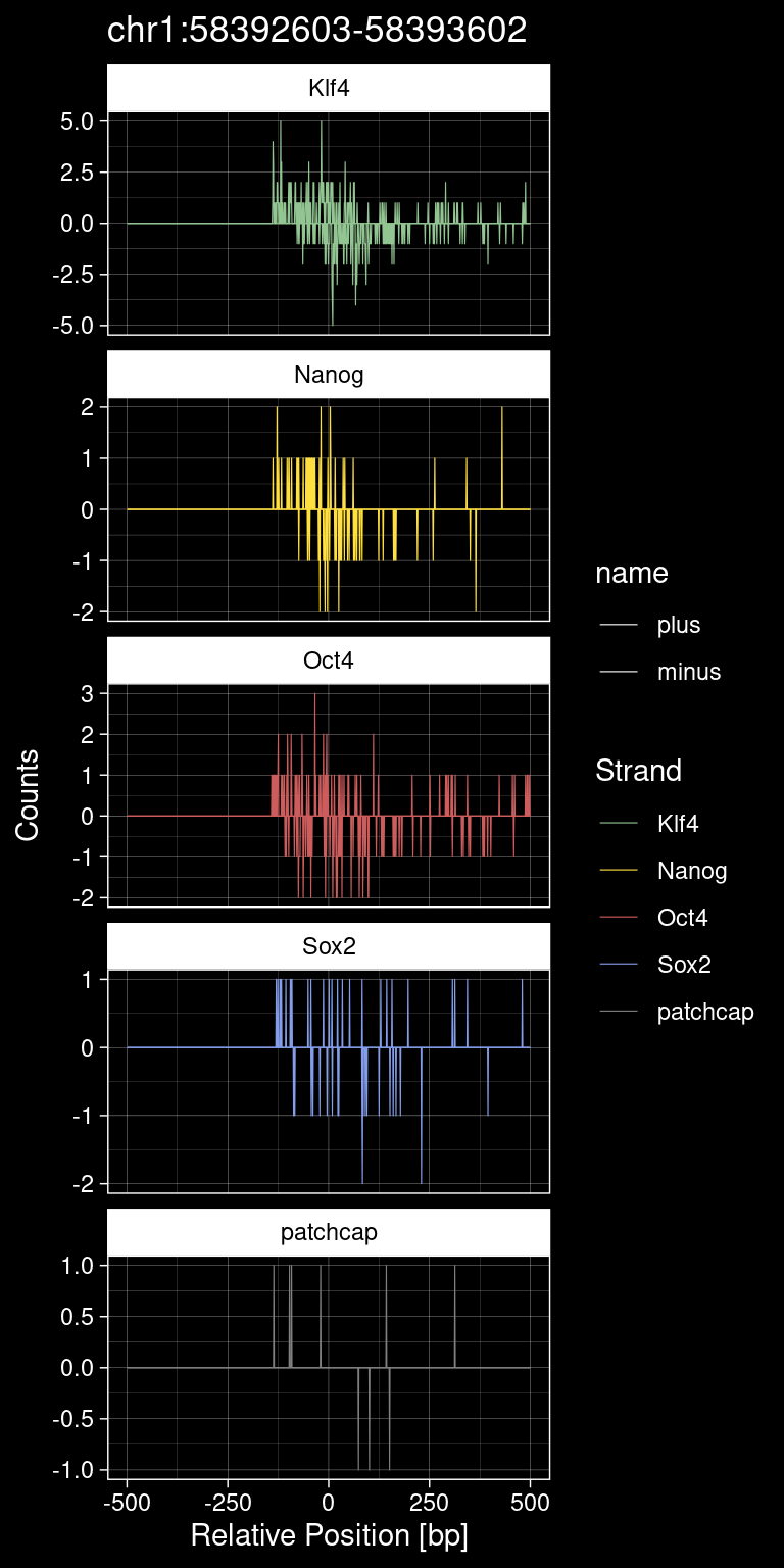
Click to view more plots
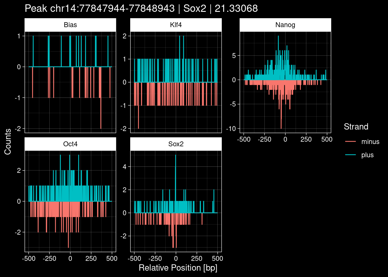
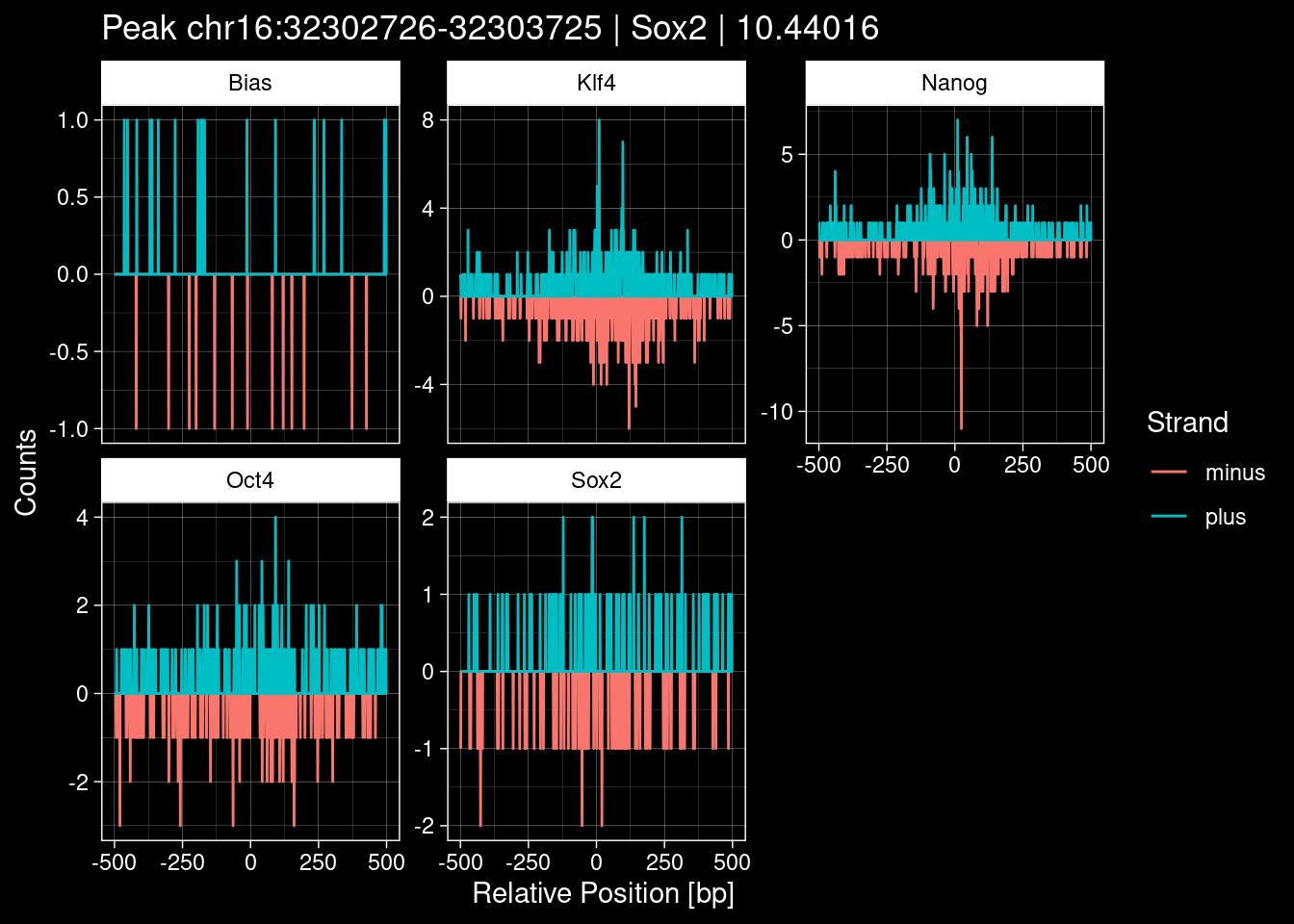
set.seed(42)
test_df <- peak_infos %>%
  as.data.frame() %>%
  dplyr::filter(set=="train") %>%
  dplyr::mutate(Region = paste0(seqnames, ":", start, "-", end)) %>%
  dplyr::group_by(TF) %>%
  slice_sample(n=5) %>%
  select(Region, TF, qValue)

purrr::walk(1:nrow(test_df), function(i) {
  test_instance <- unlist(test_df[i, ])
  purrr::map_dfr(TFs, function(tf){
  tibble::tibble(position=-499:500,
                 plus = tf_counts[[tf]]$train$pos[match(test_instance["Region"], seq_names$train), ],
                 minus = -tf_counts[[tf]]$train$neg[match(test_instance["Region"], seq_names$train), ]) %>%
    dplyr::mutate(TF = tf, p_name = test_instance["Region"])
  }) %>%
  rbind(
    tibble::tibble(position=-499:500,
                   plus = ctrl_counts$train$pos[match(test_instance["Region"], seq_names$train), ],
                   minus = -ctrl_counts$train$neg[match(test_instance["Region"], seq_names$train), ],
                   TF = "Bias", p_name = test_instance["Region"])
  ) %>%
  pivot_longer(cols=c(minus, plus)) %>%
  ggplot() +
  geom_line(aes(x=position, y=value, color=name)) +
  facet_wrap(~TF, scales="free_y") +
  ggdark::dark_theme_linedraw() +
  labs(x="Relative Position [bp]", y="Counts", color="Strand",
       title=paste0("Peak ", test_instance["Region"], " | ", test_instance["TF"],
                    " | ", test_instance["qValue"])) -> p
  print(p)
})
9 Figure 1e
9.1 From Raw Data
roi <- list("seqname"="chr1", "start"=180924752, "end"=180925152)
TFs <- c("Oct4", "Sox2", "Nanog", "Klf4")
df <-
  purrr::map_dfr(TFs, function(tf) {
    alignments <- readGAlignments(paste0("../data/chip-nexus/", tf, "/pool_filt.bam"),
                                  param = ScanBamParam(which=GRanges(paste0(roi$seqname, ":", roi$start, "-", roi$end))))
    align_pos <- alignments[strand(alignments)=="+"]
    align_neg <- alignments[strand(alignments)=="-"]

    align_pos@cigar <- rep("1M", length(align_pos))
    align_neg@start <- GenomicAlignments::end(align_neg)
    align_neg@cigar <- rep("1M", length(align_neg))

    tibble::tibble(pos=as.numeric(coverage(align_pos)$chr1[roi$start:roi$end]),
                   neg=-as.numeric(coverage(align_neg)$chr1[roi$start:roi$end]),
                   position=roi$start:roi$end,
                   TF=tf)
  }) %>%
  pivot_longer(cols=c("pos", "neg"))
df
# A tibble: 3,208 x 4
position TF name value
<int> <chr> <chr> <dbl>
1 180924752 Oct4 pos 0
2 180924752 Oct4 neg 0
3 180924753 Oct4 pos 2
4 180924753 Oct4 neg 0
5 180924754 Oct4 pos 2
6 180924754 Oct4 neg 0
7 180924755 Oct4 pos 0
8 180924755 Oct4 neg 0
9 180924756 Oct4 pos 0
10 180924756 Oct4 neg 0
# ... with 3,198 more rows
# i Use `print(n = ...)` to see more rowsdf %>%
mutate(TF = factor(TF, levels=c(TFs))) %>%
ggplot() +
geom_line(aes(x=position, y=value, col=name)) +
facet_wrap(~TF, ncol=1, scales="free_y") +
labs(x="Position", y="Counts", col="Strand") +
ggdark::dark_theme_linedraw()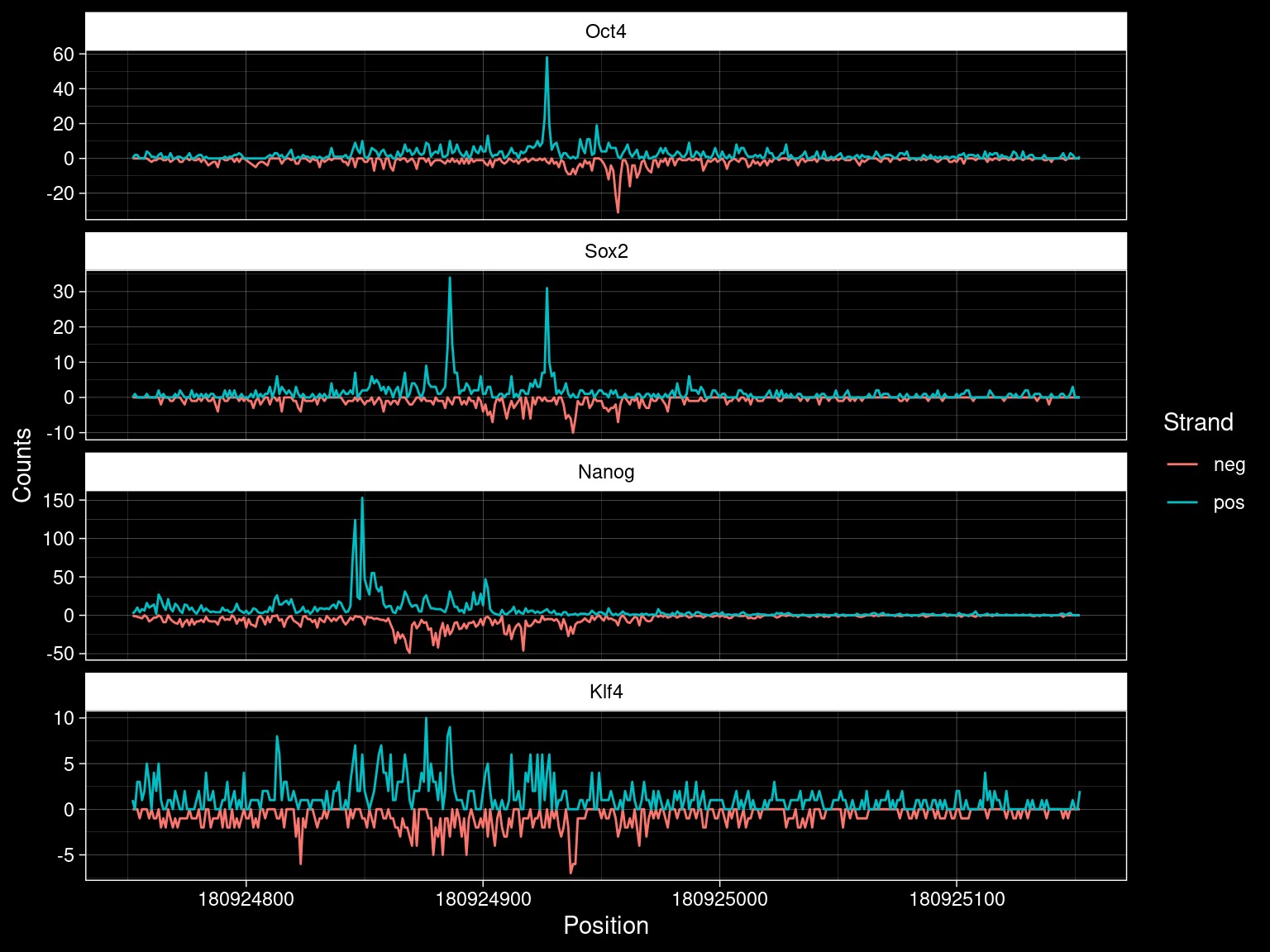
9.2 From Processed Data
roi <- list("seqname"="chr1", "start"=180924752, "end"=180925152)
roi_adjusted <- roi
roi_adjusted$start = roi_adjusted$start-1000
roi_adjusted$end = roi_adjusted$end+1000

TFs <- c("Oct4", "Sox2", "Nanog", "Klf4")
df2 <-
  purrr::map_dfr(TFs, function(tf) {
    cov_list <- list("pos" = tf_counts[[tf]]$test$pos,
                     "neg" = tf_counts[[tf]]$test$neg)
    rnames <- seq_names$test
    gr_rnames <- GRanges(rnames)

    bool_vec <-
      (as.character(gr_rnames@seqnames) == roi_adjusted$seqname &
      start(gr_rnames@ranges) >= roi_adjusted$start &
      end(gr_rnames@ranges) <= roi_adjusted$end)

    peak_index <- which(bool_vec)[1]
    peak_info <- gr_rnames[peak_index]

    diff <- 180924752 - start(peak_info@ranges) + 1
    w <- 400

    tibble::tibble(pos=cov_list$pos[peak_index, diff:(diff+w)],
                   neg=-cov_list$neg[peak_index, diff:(diff+w)],
                   position=0:400,
                   TF=tf)
}) %>%
  pivot_longer(cols=c("pos", "neg"))
df2
# A tibble: 3,208 x 4
position TF name value
<int> <chr> <chr> <dbl>
1 0 Oct4 pos 0
2 0 Oct4 neg 0
3 1 Oct4 pos 2
4 1 Oct4 neg 0
5 2 Oct4 pos 2
6 2 Oct4 neg 0
7 3 Oct4 pos 0
8 3 Oct4 neg 0
9 4 Oct4 pos 0
10 4 Oct4 neg 0
# ... with 3,198 more rows
# i Use `print(n = ...)` to see more rowsdf2 %>%
mutate(TF = factor(TF, levels=c(TFs))) %>%
ggplot() +
geom_line(aes(x=position, y=value, col=name)) +
facet_wrap(~TF, ncol=1, scales="free_y") +
labs(x="Position", y="Counts", col="Strand") +
ggdark::dark_theme_linedraw()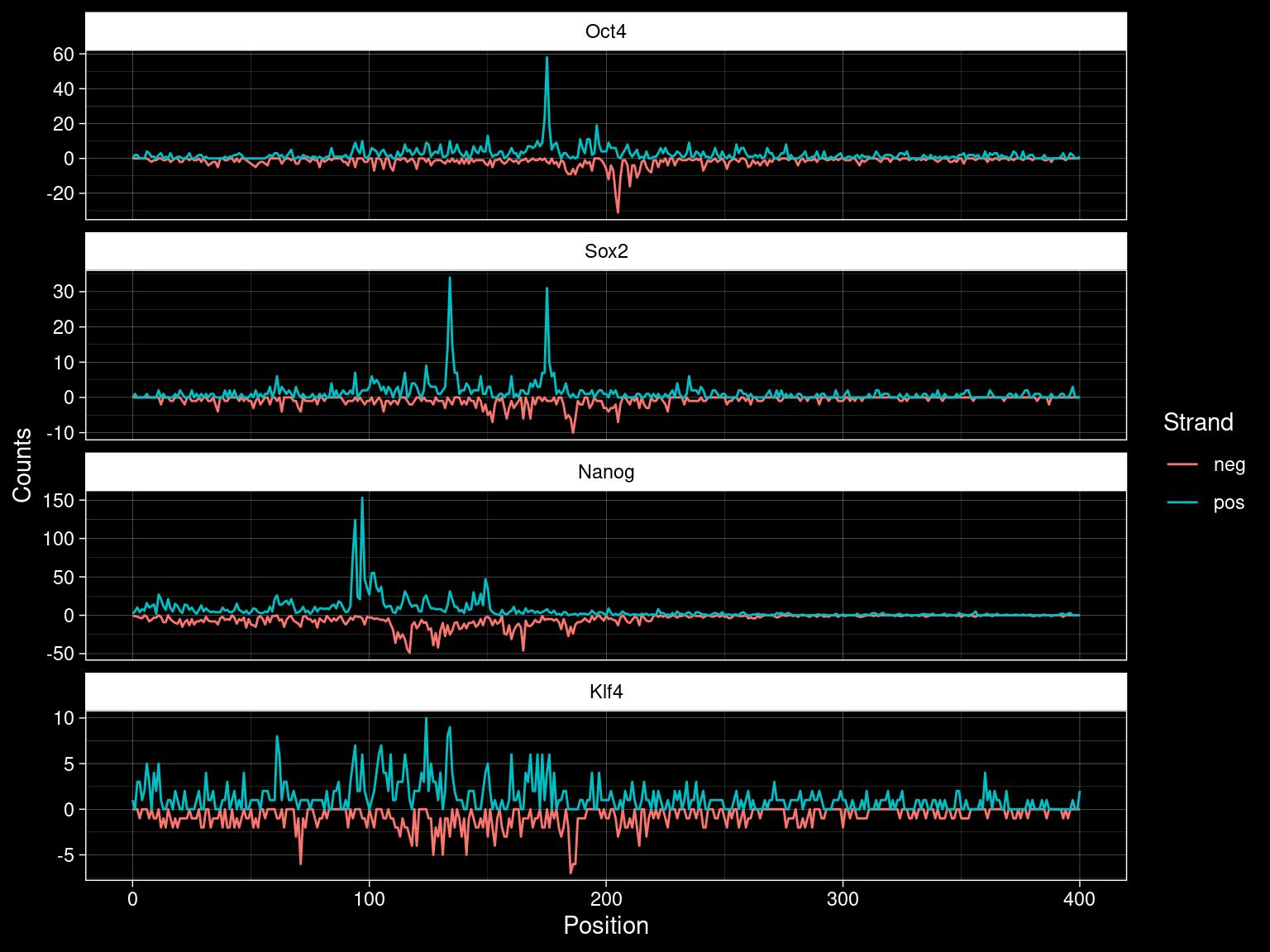
Compare.
all(df2$value == df$value)[1] TRUEall(df2$TF == df$TF)[1] TRUEall(df2$name == df$name)[1] TRUE10 Oct4-Sox2 Motif
motif <- TFBSTools::getMatrixByID(JASPAR2020, ID = "MA0142.1")
seqLogo::seqLogo(motif@profileMatrix / colSums(motif@profileMatrix))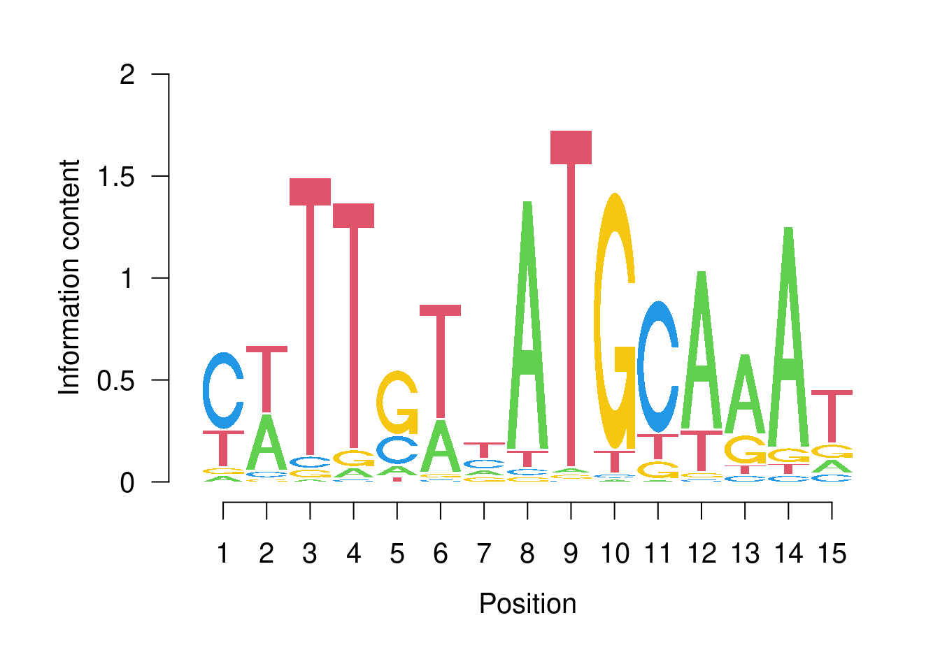
w = 400
motif_matches <- motifmatchr::matchMotifs(motif, peak_infos, genome = "mm10", out="position")[[1]] %>%
  GenomicRanges::resize(width=w, fix="center") %>%
  plyranges::filter(score > 20.8) %>%
  plyranges::arrange(score)
saveRDS(motif_matches, "/home/philipp/BPNet/input/oct4_sox2_matches.rds")
motif_matches
GRanges object with 408 ranges and 1 metadata column:
seqnames ranges strand | score
<Rle> <IRanges> <Rle> | <numeric>
[1] chr4 84528359-84528758 + | 20.8166
[2] chr4 84528359-84528758 + | 20.8166
[3] chr12 86188063-86188462 - | 20.8166
[4] chr16 23504381-23504780 + | 20.8166
[5] chr9 14619412-14619811 + | 20.8166
... ... ... ... . ...
[404] chr15 75270453-75270852 + | 23.4055
[405] chr15 80618982-80619381 - | 23.4055
[406] chr7 35617437-35617836 - | 23.4055
[407] chr8 76863085-76863484 + | 23.4055
[408] chr1 75997151-75997550 + | 23.4055
-------
seqinfo: 21 sequences from an unspecified genome; no seqlengthsmotif_matches_reduced <- GenomicRanges::reduce(resize(motif_matches, GenomicRanges::width(motif_matches + 1), "start"))
### Parallel loop over all tfs
motif_counts <- c("Oct4", "Sox2") %>%
purrr::set_names() %>%
furrr::future_map(function(tf) {
# read only from the alignment file in the given peak regions
# note: make sure that the BAM file is sorted (check for presence of ".bam.bai")
alignments <- readGAlignments(paste0("../data/chip-nexus/", tf, "/pool_filt.bam"),
param = ScanBamParam(which=motif_matches_reduced))
# split the alignment into pos and neg strand
align_pos <- alignments[GenomicRanges::strand(alignments)=="+"]
align_neg <- alignments[GenomicRanges::strand(alignments)=="-"]
# only retain first base pair of each read
align_pos@cigar <- rep("1M", length(align_pos))
align_neg@start <- GenomicAlignments::end(align_neg)
align_neg@cigar <- rep("1M", length(align_neg))
# compute the coverage per base pair
cov_list = list("pos" = GenomicAlignments::coverage(align_pos, weight = 1L),
"neg" = GenomicAlignments::coverage(align_neg, weight = 1L))
c("pos", "neg") %>%
purrr::set_names() %>%
purrr::map(function(strand) {
mtx <- matrix(data=0, ncol=w, nrow=length(motif_matches))
for (i in 1:length(motif_matches)) {
chr <- as.character(motif_matches[i]@seqnames)
position_index <- motif_matches[i]@ranges@start:(motif_matches[i]@ranges@start + w - 1)
mtx[i, ] = as.numeric(cov_list[[strand]][[chr]][position_index])
}
mtx
})
})Plotting the means per motif as in Figure 1c.
rbind(
  tibble(pos = 1:ncol(motif_counts$Oct4$pos),
         counts_pos = colMeans(motif_counts$Oct4$pos),
         counts_neg = -colMeans(motif_counts$Oct4$neg),
         TF = "Oct4"),
  tibble(pos = 1:ncol(motif_counts$Sox2$pos),
         counts_pos = colMeans(motif_counts$Sox2$pos),
         counts_neg = -colMeans(motif_counts$Sox2$neg),
         TF = "Sox2")
) %>%
  ggplot() +
  geom_line(aes(x=pos, y=counts_pos, color=TF), size=0.5) +
  geom_line(aes(x=pos, y=counts_neg, color=TF), size=0.5) +
  scale_color_manual(values=c("Oct4" = "darkred", "Sox2" = "blue")) +
  labs(x="Position [bp]", y="Coverage", color="TF") +
  ggdark::dark_theme_linedraw()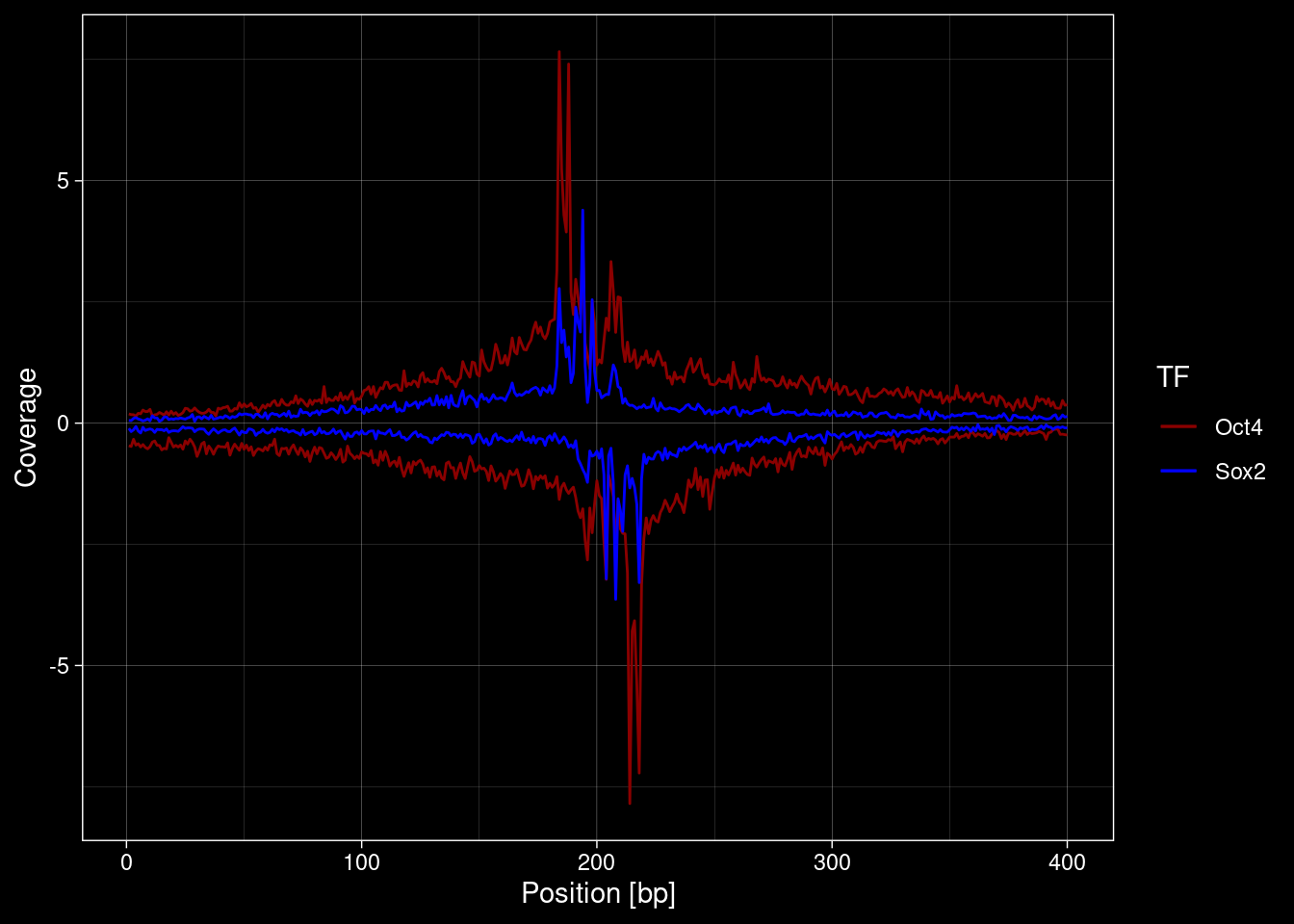
Plot the coverage per motif and per sequence as in Figure 1b
df <-
  purrr::imap_dfr(motif_counts, function(cov, tf) {
    purrr::imap_dfr(cov, function(mtx, strand) {
      purrr::map_dfr(1:nrow(mtx), function(i) {
        tibble::tibble(seq = i,
                       idx = (-w/2):(w/2 -1),
                       counts = mtx[i, ],
                       s = strand,
                       TF = tf)
      })
    })
  })
Plot via log2 FC at each position
pcount = 1
df %>%
  pivot_wider(names_from=s, values_from=counts) %>%
  dplyr::filter(TF=="Oct4") %>%
  dplyr::mutate(diff = log2(pos+pcount) - log2(neg+pcount)) %>%
  ggplot(aes(y=seq, x=idx)) +
  geom_raster(aes(fill=diff)) +
  scale_fill_gradient2(low = "blue", mid="black", high="red") +
  theme_classic() +
  labs(x = "Relative Postion [bp]", y = "Top Oct4-Sox2 Motifs", fill = "Log2 FC",
       title="Oct4") +
  ggdark::dark_mode()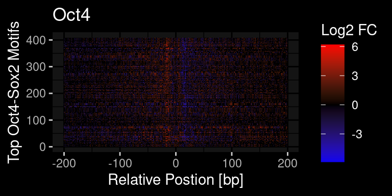
df %>%
  pivot_wider(names_from=s, values_from=counts) %>%
  dplyr::filter(TF=="Sox2") %>%
  dplyr::mutate(diff = log2(pos+pcount) - log2(neg+pcount)) %>%
  ggplot(aes(y=seq, x=idx)) +
  geom_raster(aes(fill=diff)) +
  scale_fill_gradient2(low = "blue", mid="black", high="red") +
  theme_classic() +
  labs(x = "Relative Postion [bp]", y = "Top Oct4-Sox2 Motifs", fill = "Log2 FC",
       title="Sox2") +
  ggdark::dark_mode()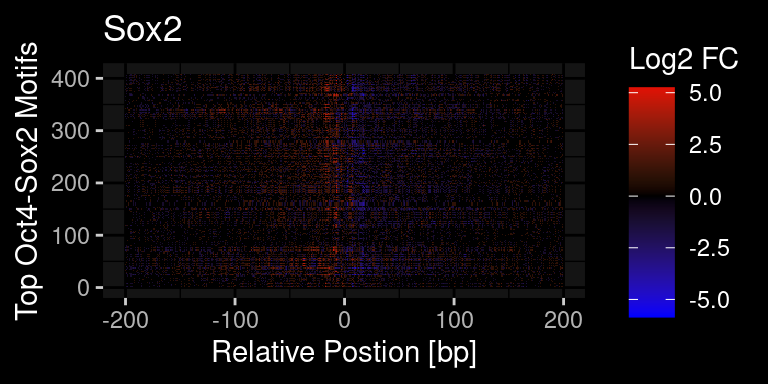
Plot via facetting
tf = "Oct4"
tmp <- df %>%
  dplyr::filter(TF==tf) %>%
  dplyr::mutate(counts = ifelse(s=="pos", counts, -counts)) %>%
  pull(counts)
df %>%
  dplyr::filter(TF==tf) %>%
  dplyr::mutate(counts = ifelse(s=="pos", counts, -counts)) %>%
  ggplot(aes(y=seq, x=idx)) +
  geom_raster(aes(fill=counts)) +
  scale_fill_gradient2(low = "blue", mid="black", high="red") +
  scale_fill_gradientn(colours = c("red", "black", "blue"),
                       values = scales::rescale(c(max(tmp), 5, 0, -5, min(tmp)))) +
  theme_classic() +
  labs(x = "Relative Postion [bp]", y = "Top Oct4-Sox2 Motifs", fill = "Log2 FC",
       title=tf) +
  ggdark::dark_mode() +
  facet_wrap(~s, ncol=1)
Scale for 'fill' is already present. Adding another scale for 'fill', which
will replace the existing scale.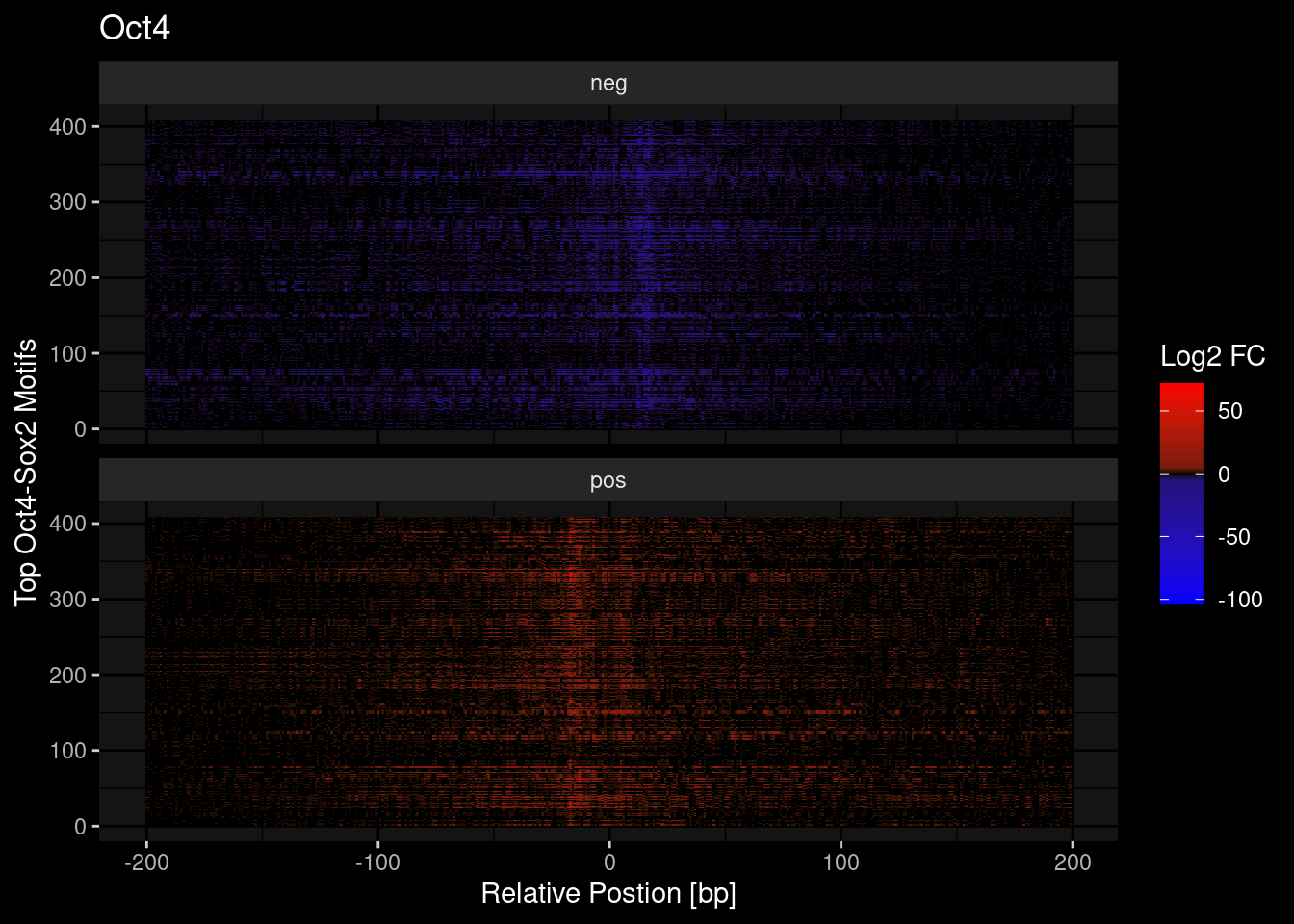
tf = "Sox2"
tmp <- df %>%
  dplyr::filter(TF==tf) %>%
  dplyr::mutate(counts = ifelse(s=="pos", counts, -counts)) %>%
  pull(counts)
df %>%
  dplyr::filter(TF==tf) %>%
  dplyr::mutate(counts = ifelse(s=="pos", counts, -counts)) %>%
  ggplot(aes(y=seq, x=idx)) +
  geom_raster(aes(fill=counts)) +
  scale_fill_gradient2(low = "blue", mid="black", high="red") +
  scale_fill_gradientn(colours = c("red", "black", "blue"),
                       values = scales::rescale(c(max(tmp), 5, 0, -5, min(tmp)))) +
  theme_classic() +
  labs(x = "Relative Postion [bp]", y = "Top Oct4-Sox2 Motifs", fill = "Log2 FC",
       title=tf) +
  ggdark::dark_mode() +
  facet_wrap(~s, ncol=1)
Scale for 'fill' is already present. Adding another scale for 'fill', which
will replace the existing scale.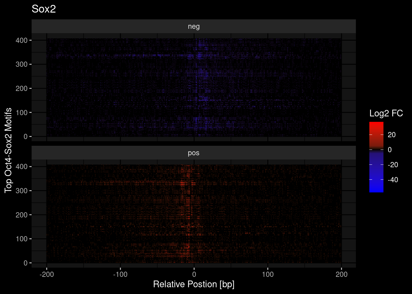
11 Appendix
11.1 Save Image
save.image(paste0(output_dir, "tmp.RData"))11.2 Session Info
sessionInfo()R version 4.2.1 (2022-06-23)
Platform: x86_64-pc-linux-gnu (64-bit)
Running under: Ubuntu 20.04.5 LTS
Matrix products: default
BLAS: /usr/lib/x86_64-linux-gnu/blas/libblas.so.3.9.0
LAPACK: /usr/lib/x86_64-linux-gnu/lapack/liblapack.so.3.9.0
locale:
[1] C
attached base packages:
[1] stats4 stats graphics grDevices utils datasets methods
[8] base
other attached packages:
[1] TFBSTools_1.34.0 JASPAR2020_0.99.10
[3] motifmatchr_1.18.0 furrr_0.3.0
[5] future_1.27.0 forcats_0.5.1
[7] stringr_1.4.0 dplyr_1.0.9
[9] purrr_0.3.4 readr_2.1.2
[11] tidyr_1.2.0 tibble_3.1.8
[13] ggplot2_3.3.6 tidyverse_1.3.2
[15] BSgenome.Mmusculus.UCSC.mm10_1.4.3 BSgenome_1.64.0
[17] BRGenomics_1.8.0 GenomicAlignments_1.32.1
[19] Rsamtools_2.12.0 Biostrings_2.64.0
[21] XVector_0.36.0 SummarizedExperiment_1.26.1
[23] Biobase_2.56.0 MatrixGenerics_1.8.1
[25] matrixStats_0.62.0 rtracklayer_1.56.1
[27] GenomicRanges_1.48.0 GenomeInfoDb_1.32.3
[29] IRanges_2.30.0 S4Vectors_0.34.0
[31] BiocGenerics_0.42.0 reticulate_1.26
loaded via a namespace (and not attached):
[1] readxl_1.4.0 backports_1.4.1
[3] plyr_1.8.7 splines_4.2.1
[5] BiocParallel_1.30.3 listenv_0.8.0
[7] digest_0.6.29 htmltools_0.5.3
[9] GO.db_3.15.0 fansi_1.0.3
[11] magrittr_2.0.3 memoise_2.0.1
[13] googlesheets4_1.0.0 tzdb_0.3.0
[15] globals_0.16.0 annotate_1.74.0
[17] modelr_0.1.8 R.utils_2.12.0
[19] colorspace_2.0-3 blob_1.2.3
[21] rvest_1.0.2 haven_2.5.0
[23] xfun_0.32 crayon_1.5.1
[25] RCurl_1.98-1.8 jsonlite_1.8.0
[27] genefilter_1.78.0 TFMPvalue_0.0.8
[29] survival_3.4-0 glue_1.6.2
[31] gtable_0.3.0 gargle_1.2.0
[33] zlibbioc_1.42.0 DelayedArray_0.22.0
[35] ggdark_0.2.1 plyranges_1.16.0
[37] scales_1.2.0 DBI_1.1.3
[39] Rcpp_1.0.9 xtable_1.8-4
[41] bit_4.0.4 httr_1.4.3
[43] RColorBrewer_1.1-3 ellipsis_0.3.2
[45] pkgconfig_2.0.3 XML_3.99-0.10
[47] R.methodsS3_1.8.2 farver_2.1.1
[49] dbplyr_2.2.1 locfit_1.5-9.6
[51] utf8_1.2.2 tidyselect_1.1.2
[53] labeling_0.4.2 rlang_1.0.4
[55] reshape2_1.4.4 AnnotationDbi_1.58.0
[57] munsell_0.5.0 cellranger_1.1.0
[59] tools_4.2.1 cachem_1.0.6
[61] cli_3.3.0 DirichletMultinomial_1.38.0
[63] generics_0.1.3 RSQLite_2.2.16
[65] broom_1.0.0 evaluate_0.16
[67] fastmap_1.1.0 yaml_2.3.5
[69] knitr_1.39 bit64_4.0.5
[71] fs_1.5.2 caTools_1.18.2
[73] KEGGREST_1.36.3 R.oo_1.25.0
[75] poweRlaw_0.70.6 pracma_2.3.8
[77] xml2_1.3.3 compiler_4.2.1
[79] png_0.1-7 reprex_2.0.1
[81] geneplotter_1.74.0 stringi_1.7.8
[83] lattice_0.20-45 CNEr_1.32.0
[85] Matrix_1.5-1 vctrs_0.4.1
[87] pillar_1.8.0 lifecycle_1.0.1
[89] bitops_1.0-7 R6_2.5.1
[91] BiocIO_1.6.0 parallelly_1.32.1
[93] codetools_0.2-18 gtools_3.9.3
[95] assertthat_0.2.1 seqLogo_1.62.0
[97] DESeq2_1.36.0 rjson_0.2.21
[99] withr_2.5.0 GenomeInfoDbData_1.2.8
[101] parallel_4.2.1 hms_1.1.1
[103] grid_4.2.1 rmarkdown_2.14
[105] googledrive_2.0.0 lubridate_1.8.0
[107] restfulr_0.0.15